This blog post will illustrate how to stream data from Twitter, aggregate it using a timed Window function and output the result to ElasticSearch, all using Apache Flink. Finally we will visualise the result using Kibana.

As always you can find the code for this example on my Github repo.

Creating SBT build file referencing latest Snapshot

Some features are only available in the very latest code base (like the Twitter Connector we will be working with today), hence I will briefly talk you through how to set up your SBT project to download the dependencies from the snapshot repository. For a detailed Flink SBT project setup guide please read my previous blog post Getting Started with Apache Flink - here I will only focus on the creating the build.sbt file.

As snapshots are not available on the standard repositories, we have to explicitly define it via a Resolver in our SBT build file:

resolvers += "apache.snapshots" at "https://repository.apache.org/content/repositories/snapshots/"

You can just browse the repo via your web browser as well to find the correct version.

Some sources show how to define the Maven dependencies, e.g.:

<dependency>
	<groupId>org.apache.flink</groupId>
	<artifactId>flink-streaming-scala_2.10</artifactId>
	<version>1.2-SNAPSHOT</version>
</dependency>

You might make the mistake to copy the artifactId value to your SBT build file like so:

libraryDependencies ++= Seq(
  "org.apache.flink" %% "flink-streaming-scala_2.10"  % "1.2-SNAPSHOT"
)

Once you compile this with SBT you will get the following warning follwed by an error:

[warn]   https://repository.apache.org/content/repositories/snapshots/org/apache/flink/flink-clients_2.10_2.10/1.2-SNAPSHOT/flink-clients_2.10_2.10-1.2-SNAPSHOT.pom
...

As you can see _2.10 is now mentioned twice, which is clearly not right! So make sure you omit it in the artifactId for your SBT build file as the Scala version (in my case 2.10) is mentioned in scalaVersion any ways already!

The correct definition looks like this:

name := "FlinkTwitterStreamCount"

version := "1.0"

scalaVersion := "2.10.4"

organization := "com.bissolconsulting"

resolvers += "apache.snapshots" at "https://repository.apache.org/content/repositories/snapshots/"

val flinkVersion = "1.2-SNAPSHOT"

libraryDependencies ++= Seq(
  "org.apache.flink" %% "flink-streaming-scala"  % flinkVersion,
  "org.apache.flink" %% "flink-clients"          % flinkVersion
)

In your project directory run sbt now and issue a compile. Once it compiles successfully, let’s add the Twitter Connector Dependency:

In the official docu we can find the Maven dependency definition:

<dependency>
  <groupId>org.apache.flink</groupId>
  <artifactId>flink-connector-twitter_2.10</artifactId>
  <version>1.2-SNAPSHOT</version>
</dependency>

This translates into SBT like so (for clarity I show the whole build.sbt file again):

name := "FlinkTwitterStreamCount"

version := "1.0"

scalaVersion := "2.10.4"

organization := "com.bissolconsulting"

resolvers += "apache.snapshots" at "https://repository.apache.org/content/repositories/snapshots/"

val flinkVersion = "1.2-SNAPSHOT"

libraryDependencies ++= Seq(
  "org.apache.flink" %% "flink-streaming-scala"  % flinkVersion,
  "org.apache.flink" %% "flink-clients"          % flinkVersion,
  "org.apache.flink" %% "flink-connector-twitter"         % flinkVersion,
  "org.apache.flink" %% "flink-connector-elasticsearch2"  % flinkVersion,
  "net.liftweb" %% "lift-json" % "3.0-M1",
  "com.github.nscala-time" %% "nscala-time" % "2.14.0"
)

Still in the SBT interactive shell type reload to reload the build configuration and then issue a clean followed by a compile.

Coding in IntelliJ IDEA

Since we appreciate the convenience that an IDE provides, we will add our SBT project as a new project to IDEA.

Creating the Twitter Source

Create the FlinkTwitterStreamCount.scala file with following content:

import java.util.Properties
import org.apache.flink.streaming.api.scala._
import org.apache.flink.streaming.connectors.twitter.TwitterSource

object FlinkTwitterStreamCount {
  def main(args: Array[String]) {

    val env = StreamExecutionEnvironment.getExecutionEnvironment

    val props = new Properties()
    props.setProperty(TwitterSource.CONSUMER_KEY, "<your-value>")
    props.setProperty(TwitterSource.CONSUMER_SECRET, "<your-value>")
    props.setProperty(TwitterSource.TOKEN, "<your-value>")
    props.setProperty(TwitterSource.TOKEN_SECRET, <your-value>")
    val streamSource = env.addSource(new TwitterSource(props))
    
    streamSource.print()
    
    env.execute("Twitter Window Stream WordCount")
  }
}

Note: Do not leave your connection details directly in the code! We will later on look at a way to externalise them.

We setup a TwitterSource reader proving all the authentication details (as described in the official docu). Compile and execute our program by clicking onto the Run button. This emits a string with random Twitter records in JSON format, e.g.:

{
  "delete": {
    "status": {
      "id": 715433581762359296,
      "id_str": "715433581762359296",
      "user_id": 362889585,
      "user_id_str": "362889585"
    },
    "timestamp_ms": "1474193375156"
  }
}

Note there is an official Flink Twitter Java example available which is worth checking out!

It’s worth noting that the Flink Twitter Connector serves a random set of tweets.

Externalising the Twitter Connection Details

Best practices first (oh well, second in the case)! We will store the Twitter token details in a properties file called twitter.properties:

twitter-source.consumerKey=<your-details>
twitter-source.consumerSecret=<your-details>
twitter-source.token=<your-details>
twitter-source.tokenSecret=<your-details>

We will add following code to our Scala file:

val prop = new Properties()
val propFilePath = "/home/dsteiner/Dropbox/development/config/ter.properties"

  try {

    prop.load(new FileInputStream(propFilePath))
    prop.getProperty("twitter-source.consumerKey")
    prop.getProperty("twitter-source.consumerSecret")
    prop.getProperty("twitter-source.token")
    prop.getProperty("twitter-source.tokenSecret")

  } catch { case e: Exception =>
    e.printStackTrace()
    sys.exit(1)
  }

val streamSource = env.addSource(new TwitterSource(prop))

Ok, that’s this done then. We can no progress with a good conscience ;)

Handling the returned JSON stream

Scala comes with a native JSON parser, however, it’s not the primary choice among developers: There are various other popular libraries out there, among them the JSON parser from the Play Framework and the Lift-JSON library from the Lift Framework. We will be using latter one. Note there is also JSON4S which builds upon Lift-JSON but promises a faster release cycles (Code on Github).

val filteredStream = streamSource.filter( value =>  value.contains("created_at"))

val parsedStream = filteredStream.map(
  record => {
    parse(record)
  }
)

//parsedStream.print()

case class TwitterFeed(
  id:Long
  , creationTime:Long
  , language:String
  , user:String
  , favoriteCount:Int
  , retweetCount:Int
)

val structuredStream:DataStream[TwitterFeed] = parsedStream.map(
  record => {
    TwitterFeed(
      // ( input \ path to element \\ unboxing ) (extract no x element from list)
      ( record \ "id" \\ classOf[JInt] )(0).toLong
      , DateTimeFormat
          .forPattern("EEE MMM dd HH:mm:ss Z yyyy")
          .parseDateTime(
            ( record \ "created_at" \\ classOf[JString] )(0)
          ).getMillis
      , ( record \ "lang" \\ classOf[JString] )(0).toString
      , ( record \ "user" \ "name" \\ classOf[JString] )(0).toString
      , ( record \ "favorite_count" \\ classOf[JInt] )(0).toInt
      , ( record \ "retweet_count" \\ classOf[JInt] )(0).toInt
    )

  }
)

structuredStream.print

So what is exactly happening here?

First we discard Twitter delete records by using the filter function.
Next we create a TwitterFeed class which will represent the typed fields that we want to keep for our analysis.
Then we apply a map function to extract the required fields and map them to the TwitterFeed class. We use the Lift functions to get hold of the various fields: First we define the input (record in our case), then the path to the JSON element followed by the unboxing function (which turns the result from a Lift type to a standard Scala type). The result is returned as a List (because if you in example lazily define the element path, there could be more than one of these elements in the JSON object). In our case, we define the absolute path the JSON element, so we are quite certain that only one element will be returned, hence we can extract the first element of the list (achieved by calling (0)). One other important point here is that we apply a Date Pattern to the created_at String and then convert it to Milliseconds (since epoch) using getMillis: Dates/Time has to be converted to Milliseconds because Apache Flink requires them in this format. We will discuss the date conversion shortly in a bit more detail.

The output of the stream looks like this:

1> TwitterFeed(787307728771440640,1476543764000,en,Sean Guidera,0,0)
3> TwitterFeed(787307728767025152,1476543764000,en,spooky!kasya,0,0)
4> TwitterFeed(787307728754442240,1476543764000,ja,あおい,0,0)
4> TwitterFeed(787307728767029248,1476543764000,ja,白芽 連合軍 ＠ 雑魚は自重しろ,0,0)

Converting String to Date

The field created_at is originally of type String. In our code we make use of the nscala-time library which is mainly a wrapper around Joda time. In your SBT build file you can reference this dependency like this:

libraryDependencies += "com.github.nscala-time" %% "nscala-time" % "2.14.0"

And you will have to add to your Scala file the following import statement:

import com.github.nscala_time.time.Imports._

We apply a formatting mask and if we need some help on this, we can take a look at the Joda Format Documentation. The create_at value looks something like this: Sun Sep 18 10:09:34 +0000 2016, so the corresponding formatting mask is EE MMM dd HH:mm:ss Z yyyy:

DateTimeFormat
.forPattern("EEE MMM dd HH:mm:ss Z yyyy")
.parseDateTime(
  ( record \ "created_at" \\ classOf[JString] )(0)
).getMillis

Creating a Tumbling Window Aggregation

While this is an interesting exercise, we cannot really send the above records like this to the windowed aggregate function: The created_at is too granular, the same goes for the id (quite likely), so any sum e.g. that we perform on retweet_count will be returned on the source data row level. One way to solve this situation is to slim down the dataset to the relevant fields: We will prepare a super simple DataStream now which only contains the language field and a constant counter. This should answer the question: How many tweets are published in a given language in 30 seconds intervals:

val recordSlim:DataStream[Tuple2[String, Int]] = structuredStream.map(
  value => (
    value.language
    , 1
    )
)

// recordSlim.print

val counts = recordSlim
  .keyBy(0)
  .timeWindow(Time.seconds(30))
  .sum(1)

counts.print

The output looks like this:

1> (et,1)
2> (tl,19)
4> (pt,72)
3> (en,433)
4> (fr,23)
2> (el,2)
1> (vi,1)
4> (in,29)
3> (no,1)
1> (ar,101)

You might want to read up on How to specify keys in the Flink functions.

Slimming down the dataset is quite often not the desired option. Another option is the use the Flink Window Functions like reduce, fold, various aggregate functions like sum etc. There is also the option to use the apply function, which provides a lot of flexibility.

While the above example is simple, this example is far from ideal. We should at least used the created_at time as the event time …

Time Types in Flink

Flink supports various time concepts:

Processing Time: This the time at which a record was processed on the machine (so in short words: machine time).
Ingestion Time: Since on a cluster data is processed on several nodes, the time on each machine might not be 100% the same. When using ingestion time, a timestamp is assigned to the data when it enters the system, so even when the data is processed on various nodes, the time will be the same.
Event Time: In a lot of cases processing and ingestion time are not ideal candidates - normally you might want to use a time which relates to the creation of the data (even time). In this case the timestamp is already part of the incoming data.

Watermarks:

To tell Flink that you want to use event time, add the following snippet:

env.setStreamTimeCharacteristic(TimeCharacteristic.EventTime)

Unsurprisingly you need to tell Flink which field your event time is (see also Generating Timestamps / Watermarks, in particular Timestamp Assigners / Watermark Generators).

Other resources:

Important: Both timestamps and watermarks are specified as milliseconds since the Java epoch of 1970-01-01T00:00:00Z. (Source: Generating Timestamps / Watermarks). This means we should define the value as type Long.

Important Info: Pre-defined Timestamp Extractors / Watermark Emitters

So while we managed to convert the created_at from String to DataTime, the missing piece is to convert this value to milliseconds since Java epoch. At the same time, we will also define a data model using a case class:

val timedStream = structuredStream.assignAscendingTimestamps(_.creationTime)

Note that the Ascending Timestamp feature does not support any late arriving data.

Creating a custom Aggregation function

We will be using the apply aggregation function, which provides a lot flexibility. Read the code inline comments below to understand how it works.

How to get window the start and end date

Currently you have to use the apply function to get hold of this data (see here for more details). The window.getStart and window.getEnd functions enable us to extract the start and end time from the Window object. In other words, for each window we have a start and end date now.

val results:DataStream[(String, Long, Long, Int)] = timedStream
  .keyBy(in => in.language)
  .timeWindow(Time.seconds(30))
  .apply
  {
    (
      // tuple with key of the window
      lang: String
      // TimeWindow object which contains details of the window
      // e.g. start and end time of the window
      , window: TimeWindow
      // Iterable over all elements of the window
      , events: Iterable[TwitterFeed]
      // collect output records of the WindowFunction
      , out: Collector[(String, Long, Long, Int)]
    ) =>
          out.collect(
            ( lang, window.getStart, window.getEnd, events.map( _.retweetCount ).sum )
           )
   }

results.print

One more point to note about this code is that specifying the key like this .keyBy("language") did not work as apparently type is not picked up for the key specification in the apply function (see also here).

As soon as we execute this code, we will get an error message similar to this one:

10/16/2016 14:35:31	TriggerWindow(TumblingEventTimeWindows(30000), ListStateDescriptor{serializer=FlinkTwitterStreamCountWithEventTime$$anon$3$$anon$1@70be965f}, EventTimeTrigger(), WindowedStream.apply(WindowedStream.scala:220)) -> Sink: Unnamed(2/4) switched to FAILED 
java.lang.RuntimeException: Record has Long.MIN_VALUE timestamp (= no timestamp marker). Is the time characteristic set to 'ProcessingTime', or did you forget to call 'DataStream.assignTimestampsAndWatermarks(...)'?
	at org.apache.flink.streaming.api.windowing.assigners.TumblingEventTimeWindows.assignWindows(TumblingEventTimeWindows.java:65)

So this tells us that we have to use the assignTimestampsAndWatermarks function - an example can be found on this blog post: Building Applications with Apache Flink Part 3: Stream Processing with the DataStream API.

val timedStream = structuredStream.assignTimestampsAndWatermarks(new AscendingTimestampExtractor[TwitterFeed] {
  override def extractAscendingTimestamp(element: TwitterFeed): Long = element.creationTime
})

If you execute the program now you will see in the results that the sum of the retweet counts is always 0. So this is not very useful. What we will do for now is a add a field called count a constant value of 1 to our structuredStream:

case class TwitterFeed(
  id:Long
  , creationTime:Long
  , language:String
  , user:String
  , favoriteCount:Int
  , retweetCount:Int
  , count:Int
)
    
val structuredStream:DataStream[TwitterFeed] = parsedStream.map(
  record => {
    TwitterFeed(
      // ( input \ path to element \\ unboxing ) (extract no x element from list)
      ( record \ "id" \\ classOf[JInt] )(0).toLong
      , DateTimeFormat
        .forPattern("EEE MMM dd HH:mm:ss Z yyyy")
        .parseDateTime(
          ( record \ "created_at" \\ classOf[JString] )(0)
        ).getMillis
      , ( record \ "lang" \\ classOf[JString] )(0).toString
      , ( record \ "user" \ "name" \\ classOf[JString] )(0).toString
      , ( record \ "favorite_count" \\ classOf[JInt] )(0).toInt
      , ( record \ "retweet_count" \\ classOf[JInt] )(0).toInt
      , 1
    )

  }
)

And then use this field in our window function to sum it up:

val results:DataStream[(String, Long, Long, Int)] = timedStream
  .keyBy(in => in.language)
  .timeWindow(Time.seconds(30))
  .apply
  {
    (
      // tuple with key of the window
      lang: String
      // TimeWindow object which contains details of the window
      // e.g. start and end time of the window
      , window: TimeWindow
      // Iterable over all elements of the window
      , events: Iterable[TwitterFeed]
      // collect output records of the WindowFunction
      , out: Collector[(String, Long, Long, Int)]
    ) =>
          out.collect(
         	( lang, window.getStart, window.getEnd, events.map( _.count ).sum )
          )
   }

The results should look like this:

1> (cs,1476642030000,1476642060000,2)
3> (ro,1476642030000,1476642060000,1)
1> (it,1476642030000,1476642060000,3)
1> (pl,1476642030000,1476642060000,5)
1> (ko,1476642030000,1476642060000,18)

So just to make sure we are still on the same page: The above stream data set shows the language code, the start and end time followed by the count/number of tweets. Just to mention it again: Due to the fact that the Apache Flink Twitter connector sources a subset of the Twitter data randomly, the result is not representative.

ElasticSearch and Kibana

We want to store our stats in a dedicated data store. InfluxDB would be a common choice, but we’ll use ElasticSearch. ElasticSearch for time-series data you might wonder? Really? Turns out it’s actually pretty good at handling time-series data based on this articel.

Installing ElasticSearch

This is fully covered in the official docu and also here.

Here an example setup for Fedora:

Download

Download the RPM file to install on Fedora.

sudo dnf install elasticsearch-2.4.0.rpm

bin/elasticsearch
curl -X GET http://localhost:9200/

OR:

sudo systemctl start elasticsearch.service

Directory Structure

Source

Type	Description	Location Debian/Ubuntu
bin files		`/usr/share/elasticsearch/bin`
config		`/etc/elasticsearch`
data	The location of the data files of each index / shard allocated on the node.	`/var/lib/elasticsearch/data`
logs	Log files location	`/var/log/elasticsearch`

Installing Kibana

Download

If you are using Fedora, download the RPM 64bit version to install on Fedora.

sudo dnf install kibana-4.6.1-x86_64.rpm
sudo systemctl start kibana.service

Getting Started

Open config/kibana.yml in an editor
Set the elasticsearch.url to point at your Elasticsearch instance
Run ./bin/kibana (or bin\kibana.bat on Windows)
Point your browser at http://localhost:5601

Directory Structure

Type	Description	Location Debian/Ubuntu
root dir		`/opt/kibana/`
bin files		`/opt/kibana/bin`
config		`/opt/kibana/config`
logs	Log files location	`???`

Installing Sense

“Sense is a Kibana app that provides an interactive console for submitting requests to Elasticsearch directly from your browser.”

Installing Sense

sudo systemctl stop kibana.service
cd /opt/kibana
sudo ./bin/kibana plugin --install elastic/sense
sudo systemctl start kibana.service

Sense is available on http://localhost:5601/app/sense.

A quick Introduction

I recommend reading the Official Getting Started Guide. There is also a forum available. Make sure that you understand the meaning of index in the context of ElasticSearch by reading this section - if you’ve never worked with ElasticSearch and you think you know what an index is in ElasticSearch, make sure you read the previously mentioned article! In essence, index is like a table in the relational world. ElasticSearch also uses an inverted index to index the document itself (ElasticSearch by default indexes every field).

With the basics out of the way, let’s test a data structure for our stream. You do not really have to explicitly create an index (table) on ElasticSearch, but you simply submit your document and tell ElasticSearch at the same time where it should be placed. If the index does not exist, it will be automatically created. Apart from the index, you also specify a type (think of it as a partition in the relational world) and a unique id, none of which have to be created upfront. The main document structure should be similar between types, but types can have some specific additional fields:

<index>/<type>/<unique-id>
# relational world equivalent
<table>/<partition>/<key>

See also here Index names must be in lower case and must not start with an underscore. Type names may be lower or upper case. The Id is a String and can be supplied or auto-generated (more details).

Action	Description
XGET	Retrieve document
XPUT	Insert or update document. Update replaces existing document
XPOST	Insert document and auto-generate id for it (see here)
XDELETE	Delete document
XHEAD	Check if document exits

Here some more useful commands

# Retrieve all documents
GET /megacorp/employee/_search
# Show all documents that have a user with a last name of Smith
GET /megacorp/employee/_search?q=last_name:Smith
# Retrieve specific fields only
GET /website/blog/123?_source=title,text

For more complex queries, you can use the Query DSL.

Defining a Schema

Flink: Using the ElasticSearch 2 connector (Sink)

In the Apache Flink 1.2 Snapshot release are ElasticSearch 1 and ElasticSearch 2 Connectors included, but they are not part of the core library, so you have to add this dependency to your build.sbt file:

"org.apache.flink" %% "flink-connector-elasticsearch2"  % flinkVersion,

Next we have to find out some configuration details:

sudo less /etc/elasticsearch/elasticsearch.yml

Search for cluster.name … you can change these details, but for my local setup I just left them as they were.

First attempt Inserting into ElasticSearch

The connection happens over TCP, ElasticSearch usually listens on port 9300.

We will create a simple example first just storing the language field in ElasticSearch - once we have this working, we implement the full solution.

First create the ES index (although I previously mentioned that you don’t really have to create an index separately we do have to do it here):

curl -XPUT 'http://localhost:9200/test'

Next let’s add this code to our Scala file:

First we set up the ElasticSearch connection details. Next we extract the language field from our stream. Finally we set up the ElasticSearch Sink. We map our stream data to a JSON object using the json.map() function.

//load data into ElasticSearch

val config = new util.HashMap[String, String]
config.put("bulk.flush.max.actions", "1")
config.put("cluster.name", "elasticsearch") //default cluster name: elasticsearch

val transports = new util.ArrayList[InetSocketAddress]
transports.add(new InetSocketAddress(InetAddress.getByName("127.0.0.1"), 9300))

// testing simple setup
val input:DataStream[String] = timedStream.map( _.language.toString)
input.print()

input.addSink(new ElasticsearchSink(config, transports, new ElasticsearchSinkFunction[String] {
  def createIndexRequest(element: String): IndexRequest = {
    val json = new util.HashMap[String, AnyRef]
    // Map stream fields to JSON properties, format:
    // json.put("json-property-name", streamField)
    json.put("data", element)
    Requests.indexRequest.index("test").`type`("test").source(json)
  }

  override def process(element: String, ctx: RuntimeContext, indexer: RequestIndexer) {
    indexer.add(createIndexRequest(element))
  }
}))

Run the program and kill it after a few seconds.

Check if the data is stored in ES:

curl -XGET 'http://localhost:9200/test/_search?pretty'

You should get data returned similar to one (after all the metadata):

}, {
  "_index" : "test",
  "_type" : "test",
  "_id" : "AVelcaqwCReiv32i2XIm",
  "_score" : 1.0,
  "_source" : {
    "data" : "fr"
  }
}, {
  "_index" : "test",
  "_type" : "test",
  "_id" : "AVelcawOCReiv32i2XIw",
  "_score" : 1.0,
  "_source" : {
    "data" : "es"
  }

Note that ElasticSearch created an id for each of our records.

Full Sink Implementation

In order to load our TimedStream into ElasticSearch, we have to make sure that ElasticSearch is aware of the field types in order to optimise performance. We will create an index mapping (a table definition in the relational world).

For further information on ElasticSearch Mapping, take a look at these documents:

Mapping
Date Format: Relevant only if your date format is different from the supported ones.
Mapping Intro

Note: For the language fields we disable the analyzer (full text indexing) function. When disabled, e.g. the word “New York” will not be broken down into “New” and “York”, so you cannot search for just “York” and get a result returns if only “New York” is available. In our case, all language values are made up of one word only, so in this case we can’t see the same impact, however, having the text fully analysed still adds overhead.

Important: When documents get added, they get indexed instantly, however refreshing the whole index is expensive. The default refresh setting is 1 second, however, if you are inserting a log of documents, you will achieve a higher throughput if you lower the refresh rate. This can be defined via the index.refresh_interval setting. See Update Index Settings and Refresh Inteveral VS Index Performance New documents will be only visible once the index is refreshed.

# delete index if already exists
  curl -XDELETE 'http://localhost:9200/tweets'
  curl -XDELETE 'http://localhost:9200/tweetsbylanguage'
# create index
  curl -XPUT 'http://localhost:9200/tweets'
  curl -XPUT 'http://localhost:9200/tweetsbylanguage'
# create mapping for lowest granularity data
curl -XPUT 'http://localhost:9200/tweets/_mapping/partition1' -d'
{
  "partition1" : {
    "properties" : {
    "id": {"type": "long"}
    , "creationTime": {"type": "date"}
    , "language": {"type": "string", "index": "not_analyzed"}
    , "user": {"type": "string"}
    , "favoriteCount": {"type": "integer"}
    , "retweetCount": {"type": "integer"}
    , "count": {"type": "integer"}
  }
  }
}'

curl -XPUT 'http://localhost:9200/tweets/_settings' -d '{
    "index" : {
        "refresh_interval" : "5s"
    }
}'
# create mapping for tweetsByLanguage
curl -XPUT 'http://localhost:9200/tweetsbylanguage/_mapping/partition1' -d'
{
  "partition1" : {
    "properties" : {
    "language": {"type": "string", "index": "not_analyzed"}
    , "windowStartTime": {"type": "date"}
    , "windowEndTime": {"type": "date"}
    , "countTweets": {"type": "integer"}
  }
  }
}'

curl -XPUT 'http://localhost:9200/tweetsbylanguage/_settings' -d '{
    "index" : {
        "refresh_interval" : "5s"
    }
}'

We will add two ElasticSearch Sinks to our Scala code: One for the low granularity data and one for the aggregate. At the same time we will also improve our windowed aggregation code a bit by assigning a case class:

val config = new util.HashMap[String, String]
config.put("bulk.flush.max.actions", "1")
config.put("cluster.name", "elasticsearch") //default cluster name: elasticsearch

val transports = new util.ArrayList[InetSocketAddress]
transports.add(new InetSocketAddress(InetAddress.getByName("127.0.0.1"), 9300))

timedStream.addSink(new ElasticsearchSink(config, transports, new ElasticsearchSinkFunction[TwitterFeed] {
  def createIndexRequest(element:TwitterFeed): IndexRequest = {
    val mapping = new util.HashMap[String, AnyRef]
    // use LinkedHashMap if for some reason you want to maintain the insert order
    // val mapping = new util.LinkedHashMap[String, AnyRef]
    // Map stream fields to JSON properties, format:
    // json.put("json-property-name", streamField)
    // the streamField type has to be converted from a Scala to a Java Type

    mapping.put("id", new java.lang.Long(element.id))
    mapping.put("creationTime", new java.lang.Long(element.creationTime))
    mapping.put("language", element.language)
    mapping.put("user", element.user)
    mapping.put("favoriteCount", new Integer((element.favoriteCount)))
    mapping.put("retweetCount", new Integer((element.retweetCount)))
    mapping.put("count", new Integer((element.count)))

    //println("loading: " + mapping)

    Requests.indexRequest.index("tweets").`type`("partition1").source(mapping)

  }

  override def process(
      element: TwitterFeed
      , ctx: RuntimeContext
      , indexer: RequestIndexer
    )
    {
      try{
        indexer.add(createIndexRequest(element))
      } catch {
        case e:Exception => println{
          println("an exception occurred: " + ExceptionUtils.getStackTrace(e))
        }
        case _:Throwable => println("Got some other kind of exception")
      }
    }
}))

case class TweetsByLanguage (
  language:String
  , windowStartTime:Long
  , windowEndTime:Long
  , countTweets:Int
)

val tweetsByLanguageStream:DataStream[TweetsByLanguage] = timedStream
  // .keyBy("language") did not work as apparently type is not picked up
  // for the key in the apply function
  // see http://stackoverflow.com/questions/36917586/cant-apply-custom-functions-to-a-windowedstream-on-flink
  .keyBy(in => in.language)
  .timeWindow(Time.seconds(30))
  .apply
  {
    (
      // tuple with key of the window
      lang: String
      // TimeWindow object which contains details of the window
      // e.g. start and end time of the window
      , window: TimeWindow
      // Iterable over all elements of the window
      , events: Iterable[TwitterFeed]
      // collect output records of the WindowFunction
      , out: Collector[TweetsByLanguage]
    ) =>
      out.collect(
        // TweetsByLanguage( lang, window.getStart, window.getEnd, events.map( _.retweetCount ).sum )
        TweetsByLanguage( lang, window.getStart, window.getEnd, events.map( _.count ).sum )
      )
  }

// tweetsByLanguage.print

tweetsByLanguageStream.addSink(
  new ElasticsearchSink(
    config
    , transports
    , new ElasticsearchSinkFunction[TweetsByLanguage] {

      def createIndexRequest(element:TweetsByLanguage): IndexRequest = {
        val mapping = new util.HashMap[String, AnyRef]

        mapping.put("language", element.language)
        mapping.put("windowStartTime", new Long(element.windowStartTime))
        mapping.put("windowEndTime", new Long(element.windowEndTime))
        mapping.put("countTweets", new java.lang.Integer(element.countTweets))


        // println("loading: " + mapping)
        // problem: wrong order of fields, id seems to be wrong type in general, as well as retweetCount
        Requests.indexRequest.index("tweetsbylanguage").`type`("partition1").source(mapping)

      }

      override def process(
        element: TweetsByLanguage
        , ctx: RuntimeContext
        , indexer: RequestIndexer
        )
        {
          try{
            indexer.add(createIndexRequest(element))
          } catch {
            case e:Exception => println{
              println("an exception occurred: " + ExceptionUtils.getStackTrace(e))
            }
            case _:Throwable => println("Got some other kind of exception")
        }
      }
    }
  )
)

So what’s happening here? In a nutshell:

We set up the connection details.
We add a sink. At this point we have to convert our stream data to a JSON representation. We then request ElasticSearch to store the JSON objects in a predefined index and type.

If for some reason you cannot find the data on ElasticSearch (when you program executed without any errors), consult the ElasticSearch Log:

less /var/log/elasticsearch/elasticsearch.log

In my case I found a message shown below because there was a type mismatch (not because the order of the field matters):

[2016-10-11 17:45:09,306][DEBUG][action.bulk              ] [Sleek] [twitter][3] failed to execute bulk item (index) index {[twitter][languages][AVe0oir-LpV6XBRrSKbo], source[{"creationTime":"1476204303000","language":"ko","id":"7.8588392611606938E17","retweetCount":"0.0"}]}
MapperParsingException[failed to parse [language]]; nested: NumberFormatException[For input string: "ko"];

Note: Elements in a JSON object are by definition unordered (as discussed here and here). JSON libraries can arrange the elements in any particular order (which means not necessarily in the order we specified them). The ElasticSearch Mapping we created earlier on does not require the elements to be in a given order either. This is important to understand for readers coming from the relational database world, where fields have to be inserted in a predefined order into a table. However, if for some reason you want to maintain the insert order in the JSON object, in Scala, we can use an immuatable ListMap to just achieves this (as well as the Java LinkedHashMap).

Check if the data is stored in ES:

curl -XGET 'http://localhost:9200/tweets/_search?pretty'

The result should look something like this (after all the metadata):

}, {
  "_index" : "tweets",
  "_type" : "partition1",
  "_id" : "AVftNj2olHqgUwl-blye",
  "_score" : 1.0,
  "_source" : {
    "creationTime" : 1477153522000,
    "count" : 1,
    "language" : "en",
    "id" : 789865239164571649,
    "user" : "nnn",
    "retweetCount" : 0,
    "favoriteCount" : 0
  }
} 

And let’s do the same for the aggregate:

curl -XGET 'http://localhost:9200/tweetsbylanguage/_search?pretty'

The result should look something like this (after all the metadata):

}, {
  "_index" : "tweetsbylanguage",
  "_type" : "partition1",
  "_id" : "AVftP2zFlHqgUwl-bl-V",
  "_score" : 1.0,
  "_source" : {
    "windowStartTime" : 1477154100000,
    "windowEndTime" : 1477154130000,
    "countTweets" : 1,
    "language" : "hi"
  }
}

This is all looking quite promising so far!

If you interested in how many documents/JSON objects we have inserted so far into ElasticSearch and how much disk space they consume, run the following command:

$ curl 'localhost:9200/_cat/indices?v'
health status index            pri rep docs.count docs.deleted store.size pri.store.size 
yellow open   tweets             5   1       7598            0      1.4mb          1.4mb 
yellow open   tweetsbylanguage   5   1        308            0    132.7kb        132.7kb 

Visualising results with Kibana

It’s been quite a journey! If you made it until this point I applaud your determination. Don’t you worry, we have still one more exciting destination ahead of us: Visualising the results generated by our Flink windowing function.

Note: Visualisations in Kibana are more geared towards aggregated data. You can define the type of aggregation via Kibana and the data will be aggregated on ElasticSearch. Since our data should be displayed as is (no aggregation), we kind of have to trick the system a bit.

If you haven’t done already, fire up Kibana and access the UI via http://localhost:5601.
Navigate to Settings > Indices. If haven’t set up in index before, you will directly see the Configure an index pattern page, otherwise click Add New.
Make sure that Index contains time-based events is ticked.
Specify tweetsbylanguage as index name.
Choose windowStartTime from the drop-down list as time-field name.
Finally click Create.

On the next page you see an overview of all the fields:

Click on Discover in the top menu bar and you will be able to search trough the documents we just loaded:

Next click on Visualise in the top menu bar and choose a Line Chart followed by From new search.

How to create a Multi-Line Chart

Setup Data:

Y-Axis: Add Metrics, Aggregation: Sum, Field: countTweets, remove other metrics.
Buckets:
- X-Axis, Aggregation: Date Histogram, Interval: Second
- Add sub-buckets: Split Lines, Sub-Aggregation: Terms, Field: language, Order by: metric: Sum of countTweets, Order: Descending, Size: 5

Note: We specified sum in the metric of the sub-buckets. We could have chosen any other aggregation as well, since what we specified will basically return our data as is (no aggregation should take place). This is what I mentioned earlier on about “tricking the system”.

Save the chart now.

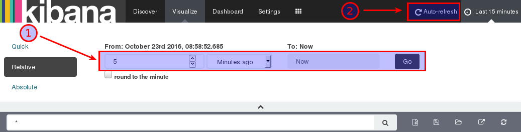
Important: In the top right hand corner you have an option to choose the time period you want to see the data for. The default in my case was set to last 15 Minutes. Just click on it and choose Relative and a suitable time period (e.g. 15min ago to now).

Enabling auto-refresh:

In the right top hand corner click on the watch icon and set the time filter to relative and choose the last 5 minutes to be displayed:

Next click on the Auto-refresh icon (situated in the top menu bar on the righ hand side) and set the refresh rate to 30 seconds:

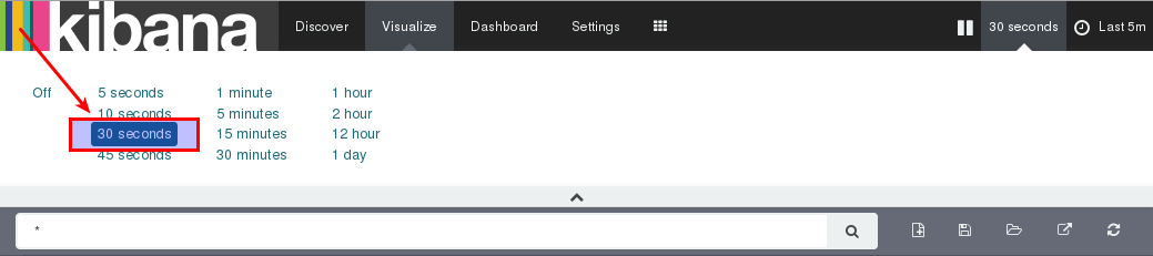
You chart will now be kept up-to-date.

Granted this is not the best choice of chart for displaying this data, but you can improve on this.

Creating SBT build file referencing latest Snapshot

Coding in IntelliJ IDEA

Creating the Twitter Source

Externalising the Twitter Connection Details

Handling the returned JSON stream

Converting String to Date

Creating a Tumbling Window Aggregation

Time Types in Flink

Creating a custom Aggregation function

ElasticSearch and Kibana

Installing ElasticSearch

Directory Structure

Installing Kibana

Directory Structure

Installing Sense

A quick Introduction

Defining a Schema

Flink: Using the ElasticSearch 2 connector (Sink)

First attempt Inserting into ElasticSearch

Full Sink Implementation

Visualising results with Kibana

Additional Sources