In this article we will have a look at various approaches on how to create snapshot tables with varying degrees of flexibility. We will start by taking a brief look at the classic Kimball approaches, then discuss a different approach for a Big Data environment and finally take a look at an alternative approach which I came up with. This article is more of a theoretical nature - initially I tried to include some practical examples, but the article was just getting way too long, so I cut it back to the essential points.
Classic Kimball Approaches
Both the snapshot as well as the accumulating snapshot rely on a fact table. You can think of them as alternative views on the same data, which allow to answer a different set of questions.
Snapshot
A snapshot allows us to easily check at which stage a certain item is on a given day: A classic example is an item being delivered from your online merchant to your doorstep. It’s a predefined process with given steps. A classic Kimball style snapshot would list the ID of your order, any dimensions, a date or timestamp for each of the steps (e.g. Package ready to be dispatched, Arrived at local distribution centre etc) and there would be a counter of 1 for each of the steps completed. The table row gets updated as the delivery progresses. This works fine for processes that are more of a static nature.
Here an extremely simplified example: The object with id 20 just entered step 1 in our process, hence we insert a new record populating the respective fields:
| id | dim_a | step_1_started_tk | step_2_started_tk | step_1_count | step_2_count |
|---|---|---|---|---|---|
| 20 | aaa | 20150602 | NULL |
1 | NULL |
Two days later when the objects enters step 2 of our process we have to update the snapshot table with the timestamp and count:
| id | dim_a | step_1_started_tk | step_2_started_tk | step_1_count | step_2_count |
|---|---|---|---|---|---|
| 20 | aaa | 20150602 | 20150604 | 1 | 1 |
Important: Dimensional values which were originally inserted for one particular record never get updated! So the value of
dim_ain the above example must not change at any point. The same principles as for the standard fact table apply: No data gets overwritten at any point. It’s a write once process (In the case of the snapshot on a cell level).
If the process is of a more flexible nature, e.g. it’s possible to jump one or several steps back and forward (even several times), then pursuing the Kimball style snapshot approach might be quite a challenge/impossible.
Accumulating Snapshot
Snapshot tables allow us to answer the question How many items entered step/stage X on a certain day?, however, they do not allow us to answer the question How many items do we have in a given step/stage of our process on a given day?: This is what accumulating snapshots are for.
| snapshot_date_tk | dim_a | dim_b | quantity_on_hand_eod |
|---|---|---|---|
| 20150603 | aaa | bbb | 234 |
The quantity on hand is usually measured at the end of the day.
Accumulating Snapshot saves reporting solutions the computing intensive task of having to calculate for each day how many objects entered and exited a certain stage/step since the very beginning.
The ETL process has less to do as well to create a new record: We only have to look at the previous day’s accumulative quantity and then add all the new objects entering the step/stage and subtract all the objects leaving this step/stage. So it is a fairly easy calculation as well.
Creating an event table
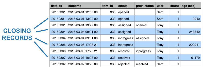
On a recent project the task was to store any event in a workflow on Hadoop. As most of you will know, Hadoop HDFS was not originally designed for updates, hence we had to resort to an alternative strategy - which was suggested by Nelson Sousa: The idea is to negate the last event once a new event arrives. The original event has a count of 1 whereas the negating/closing record of the same event has a count of -1. When you sum the records, the result will be 0.
Another requirement was that we can record any event: The workflow is not necessarily sequential. Items can jump back and forth several steps several times. This means that Kimball’s accumulating snapshot approach cannot be applied.
The basic algorithm will create a closing record for each event once a new one arrives. The closing record’s date will be the same as the one of the next event:
A second ETL process creates the accumulating snapshot, which we will discuss next.
Creating the Accumulating Snapshot
In order to be able to analyse the amount of items in a certain state on a given day, we have to create an accumulating snapshot table. The setup is similar to the one of bank statement: There is a balance and the difference to the previous balance is shown (in form of transactions). Hence there is no need to recalculate everything since the opening of bank account.
Filling the gaps: The important point to consider is that for a daily snapshot we have to create daily records even if there is no measure available for this particular day and the given combination of dimensions. The fillings are highlighted in the below screenshot in blue:
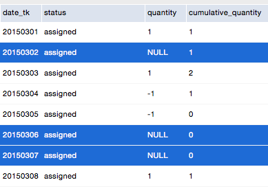
A more sensible approach is to not create fillers once the cumulative sum of a given combination of dimensions reaches zero - this will safe you some disk space.
A simple strategy to create these fillings in the ETL is to calculate the difference in amount of days between the current record and the next record and subtract minus 1. Then you can use this number to clone the current record. Care must be taken to set any measures to NULL in the clones (apart from the cumulative measures).
Creating the Cube Definition
Writing the Mondrian OLAP Schema for the snapshot and accumulating snapshot tables is quite straight forward. The one noteworthy point is that we should create a derived dimension called Flow (based on our +1 and -1 counts) in order to better show the in and out movement. Another important point is that the end users have to be educated to only analyse accumulating snapshot figures on a daily level, as they will not roll up to a higher level (unless you fancy implementing semi-additive measures, which automatically picks the beginning of the month e.g. if you are on a monthly level - this can be quite performance intensive though).
Sample Analysis
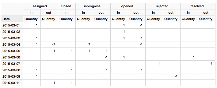
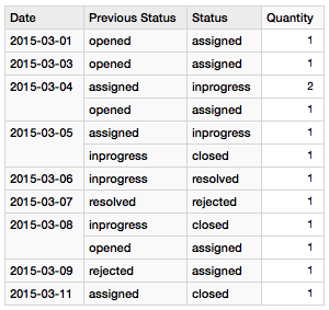
A very simple report will show the amount of issues added and removed from a certain status on a given day:
The next report is a bit similar, but we set following filters:
- Show all Statuses except
Opened - Show all statuses for Flow
inonly
Our sample dataset is extremely small, but in real world scenarios you can take the output of the above query for just one day and display it in a Sankey or Alluvial Diagram. Here is an example based around our use case, just with a bit more data:
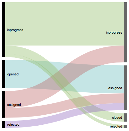
The above diagram was quickly created with RAW - a good way to prototype this type of chart. You can later on implement this kind of chart in a Pentaho CDE dashboard.
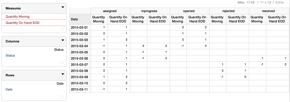
And finally we want to understand how many items there are each day in a given status, which can be answered by our Accumulating Snapshot cube:
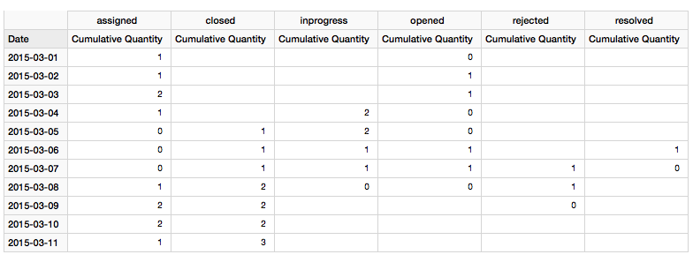
2015-03-01 shows 0 items as in Status opened. The reason for this is that the snapshot represents the state at the end of the day: One item was opened on 2015-03-01 and assigned on the same day, hence our snapshot shows 0 for opened and 1 for assigned.
Creating an Accumulating Snapshot Table
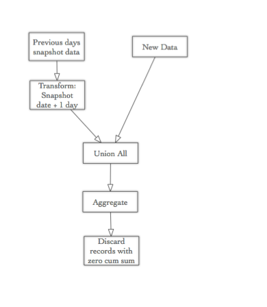
Basic Strategy - Processing One Day at a time
- We get the snapshot data of the previous day (so that we have access to the cumulative figure) and increase the snapshot date by one day (so that it has the same snapshot date as the new data). We rename the cumulative sum field to the same name as the measure field in the new dataset (see 2.), so that we can easily aggregate them.
- We get one day worth of new data and transform it to have exactly the same field structure as the snapshot dataset.
- We merge the two datasets in a SQL style
UNION ALLfashion. - Now we just have to aggregate the merged dataset by all dimensional columns and we have the new cumulative sum.
- Filter out the records which have a zero cumulative sum and discard them (if you want to save storage space).
Basic Strategy - Processing several days at once
The approach below assumes that you do not have any late arriving data.
- From the existing accumulative snapshot data, get the records for the last/most recent date as we have to have access to the cumulative quantity.
- Get the new data (all days).
- Merge streams in a SQL
UNION ALLfashion. - Sort the data in ascending order.
- Create the cumulative sum.
- From the new data we require the maximum date (across any combination of dims).
- Create Fillers: Calculate the required number of clones between the given record and the next one (in the same dimensional category). If there is no record available for that particular dimensional category for the last day within this dataset, use the maximum date from step 5 to calculate the additional clones. Finally, based on the previously derived required clones number, clone the records (hence creating the fillers).
- Discard the existing accumulative snapshot data from step 1.
This is only a very rough outline, there are many more steps required to make this work properly.
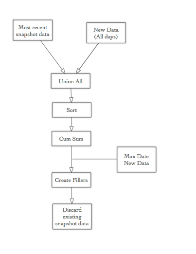
Why do we need the max date of the new data? Because we have to create filler records for any combination of dimensions until this date in case there is no measure for them available. E.g. we might have measures for category X until the most recent date but for category Y we might only have data until 2 days earlier. So even though no changes happened for category Y, we still have to create records for it (in the ideal case only if the cumulative sum is not zero).
It is worth noting that if there is a certain category (combination of dims) in the existing snapshot data but no corresponding new data, we have to keep on creating records for them in the snapshot table for each day (create clones). But this is quite often an overkill, as I don’t consider it necessary to show records when there is a cumulative sum of 0.
For all categories (combinations of dims) that we create clones for for each day, the cumulative sum will be the same and the standard sum/quantity has to be set to 0.
In a nutshell: If there are no new measures for a given day, a snapshot table still has to show a record (if that combination of dims showed up in the past).
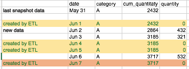
The example above (shown in the screenshot) illustrates some of the considerations we have to take:
- Gaps in data (rows with green font)
- No data between 31 May and Jun 2 (rows with yellow background colour)
- No data between 3rd and 6th June (most recent date in the example) (rows with red background colour): For other categories we have data up to the 7th June, so we have to create an extra record for this category / combination of dimensions.
Complications When Adding Age (in Days or Working Days)
THIS SECTION IS WORK IN PROGRESS AND MIGHT BE INCOMPLETE
On one of the project I was working the requirement was to be able to analyse how many working days a Jira issue was in a certain state. Here an example from fact_events (the table which holds the +1 and -1 event entries):
| issue_id | state | datetime | event_count |
|---|---|---|---|
| 288 | Opened | 2015-09-01 12:31:00 | 1 |
| 288 | Opened | 2015-09-03 10:11:00 | -1 |
Adding the age in days or working days adds further complication to creating a snapshot, as we will see shortly:
| issue_id | state | datetime | event_count | age (days) |
|---|---|---|---|---|
| 288 | Opened | 2015-09-01 12:31:00 | 1 | 0 |
| 288 | Opened | 2015-09-03 10:11:00 | -1 | 2 |
Note: Adding a counter for age working days to
fact_eventsis a bit trickier. An efficient way to calculate the difference in working days between one event and the next is to add to thedim_datetable a counter of working days since first day present in your date dimension. This way you only have to subtract the working days counter of the current event date from the next one.
In our snapshot ETL, in memory, we would expand the previously shown dataset to the following:
| issue_id | state | datetime | event_count | age (days) |
|---|---|---|---|---|
| 288 | Opened | 2015-09-01 12:31:00 | 1 | 0 |
| 288 | Opened | 2015-09-02 00:00:00 | 0 | 1 |
| 288 | Opened | 2015-09-03 10:11:00 | -1 | 2 |
Now the problem is that our event count of +1 and -1 are not representative any more, because we introduced a deeper granularity by adding the age in days. To correct this, we would have to create a dataset like this:
| issue_id | state | datetime | age (days) | event_count |
|---|---|---|---|---|
| 288 | Opened | 2015-09-01 12:31:00 | 0 | 1 |
| 288 | Opened | 2015-09-02 00:00:00 | 0 | -1 |
| 288 | Opened | 2015-09-02 00:00:00 | 1 | 1 |
| 288 | Opened | 2015-09-03 10:11:00 | 1 | -1 |
| 288 | Opened | 2015-09-03 10:11:00 | 2 | 1 |
| 288 | Opened | 2015-09-03 10:11:00 | 2 | -1 |
| 288 | Assigned | 2015-09-03 10:11:00 | 0 | 1 |
Now the key is made up of issue_id, state, datetime and age (days), hence the Jira issue can enter and exit this detailed state.
If the requirement is to use working days, the strategy is still the same, however, one point worth noting is, that the some key values can exist across several days, e.g. a weekend:
| issue_id | state | datetime | age (working days) | event_count |
|---|---|---|---|---|
| 288 | InProgress | 2015-09-04 13:22:00 | 0 | 1 |
| 288 | InProgress | 2015-09-05 00:00:00 | 0 | 0 |
| 288 | InProgress | 2015-09-06 00:00:00 | 0 | 0 |
| 288 | InProgress | 2015-09-07 00:00:00 | 0 | -1 |
| 288 | InProgress | 2015-09-07 00:00:00 | 1 | 1 |
| 288 | InProgress | 2015-09-08 00:00:00 | 1 | -1 |
| 288 | InProgress | 2015-09-08 10:11:00 | 2 | 1 |
| 288 | InProgress | 2015-09-08 10:11:00 | 2 | -1 |
| 288 | UnderReview | 2015-09-08 10:11:00 | 0 | 1 |
So this is getting fairly complex now. We have to find a better strategy that works with our initial fact events table data:
How about just flagging the rows if they are on hand instead of creating the enter-exit (+1 -> -1) combos and using a standard Sum instead of an Cumulative Sum aggregation? Would this not be easier?
| issue_id | state | datetime | event_count | age (days) | quantity on hand |
|---|---|---|---|---|---|
| 288 | Opened | 2015-09-01 12:31:00 | 1 | 0 | 1 |
| 288 | Opened | 2015-09-02 00:00:00 | 0 | 1 | 1 |
| 288 | Opened | 2015-09-03 10:11:00 | -1 | 2 | 0 |
In this case we have to create only one filler record a day for each unique key combination. One important point to consider is that we have to ignore intra-day state changes, e.g.:
| issue_id | state | datetime | event_count | age (days) | quantity on hand |
|---|---|---|---|---|---|
| 277 | Opened | 2015-09-01 12:31:00 | 1 | 0 | 0 |
| 277 | Opened | 2015-09-01 13:33:00 | -1 | 0 | 0 |
| 277 | Assigned | 2015-09-01 13:33:00 | 1 | 0 | 1 |
| 277 | Assigned | 2015-09-02 11:23:00 | -1 | 1 | 0 |
| 277 | InProgress | 2015-09-02 11:23:00 | 1 | 0 | 1 |
Note: As Jira issue 277 gets opened and then assigned on the same day, the entering and exit records of state
Openedhave bothquantity on handset to0.
In most cases we do not want to keep the same granularity in the snapshot table as in the fact events table. Usually we would at least get rid of the issue_id.
Why we cannot aggregate straight away
The problem when we aggregate the input data straight away is that we lose track of how many clones/fillers are required. The number of required clones has to be determined at the lowest granularity (before aggregating the data). To illustrate this problem, let’s have a look at this highly simplified example:
| Date | Issue_ID | Status |
|---|---|---|
| 2015-09-01 | 66 | Opened |
| 2015-09-03 | 66 | Assigned |
| 2015-09-01 | 77 | Opened |
| 2015-09-05 | 77 | Assigned |
So let’s aggregate this a bit:
| Date | Status | quantity on hand |
|---|---|---|
| 2015-09-01 | Opened | 2 |
| 2015-09-03 | Assigned | 1 |
| 2015-09-05 | Assigned | 1 |
Now we don’t know any more how these records are related. How many clones do we have to create for each one of these input rows? The solution is to add a new field called something like number of required clones to the input dataset. It is important to remember that this all happens on the lowest granularity (same granularity as the fact_events table), however, we do not include any other fields than the ones that we want to aggregate on later on.
| Date | Status | Required Clones | quantity onhand |
|---|---|---|---|
| 2015-09-01 | Opened | 1 | 1 |
| 2015-09-03 | Assigned | 2 | 1 |
| 2015-09-01 | Opened | 3 | 1 |
| 2015-09-05 | Assigned | 0 | 1 |
Note: You might wonder why for the second record two clones are required? This is because the maximum date of the input dataset is
2015-09-05and for each composite key we have to create a row until this date!
Based on this dataset we can create the number if required clones:
| Date | Status | quantity on hand | data source |
|---|---|---|---|
| 2015-09-01 | Opened | 1 | input data |
| 2015-09-02 | Opened | 1 | cloned later by ETL |
| 2015-09-03 | Assigned | 1 | input data |
| 2015-09-04 | Assigned | 1 | cloned later by ETL |
| 2015-09-05 | Assigned | 1 | cloned later by ETL |
| 2015-09-01 | Opened | 1 | input data |
| 2015-09-02 | Opened | 1 | cloned later by ETL |
| 2015-09-03 | Opened | 1 | cloned later by ETL |
| 2015-09-04 | Opened | 1 | cloned later by ETL |
| 2015-09-05 | Assigned | 1 | input data |
Once the ETL process created in memory the required clones (ideally in memory), we can aggregate this result:
| Date | Status | quantity on hand |
|---|---|---|
| 2015-09-01 | Opened | 2 |
| 2015-09-02 | Opened | 2 |
| 2015-09-03 | Assigned | 1 |
| 2015-09-03 | Opened | 1 |
| 2015-09-04 | Assigned | 1 |
| 2015-09-04 | Opened | 1 |
| 2015-09-05 | Assigned | 2 |
Important Rules
There are some rules to consider when aggregating the fact event data:
- The fact events table needs an additional
age_in_daysfields so that we can derived the required number of clones for the snapshot from it. - We have to exclude intraday records from our input dataset for the snapshot ETL. The snapshot is taken at the end of the day, so if a given
issue_identers and exists a status within the same day, we do not want to count it as on hand. It is important to understand that we for any given day and composite key combination there must be only one record in input data set: The item can only be in one state at the end of the day!
Important: To determine an intraday change, we get the datetime of the next status/event. We cannot just check if
next_datetime - datetimeis bigger than one day, as thenext_datetimecould be on the next day theoretically, but what we want to make sure is is to count the on hands issues at the end of the given day, so the correct way to do this is to compare that date part ofdatetimewith the date part ofnext_datetime. If both dates are the same, then we must consider it as an intraday change! But you might have realised that we don’t need an additionalis_intraday_changefield in the fact events table: This is because we can just filter out the record pairs as well that have a negating record withage_days = 0.
| issue_id | state | datetime | event count | age days |
|---|---|---|---|---|
| 367 | Opened | 2015-09-02 12:32:00 | 1 | 0 |
| 367 | Opened | 2015-09-02 13:11:00 | -1 | 0 |
- We only want to keep the non-intra-day negating (exiting) records (
-1) to create the fillers in the ETL. Once the fillers are created, we discard these records.
Creating an efficient input query for the ETL
The challenge is to figure out which record is the most recent open one: For this particular record we have to apply a different logic to calculate the required number of clones. We could write a performance intensive subquery to return these records, but let’s see if we can come up with a better approach:
Solution:
- Import data in reverse order
- Keep first
+1record (all records that entered a new status). - Filter out all the other
+1s - Use the
-1records to get the the age_days, which we can use to create the required number of clones.age_daysstart at0, so we can use it 1 to 1 for the number of required clones. For the ones that just entered a new status (latest+1records), we use the maximum date of the whole input dataset to calculate the number of clones (so this basically boils down to:age_days = max_date_input_data - event_start_date). Then we replace theevent_start_datewith themax_date_input_datafor these records. Now all records have the same logic.
Example:
Fact Events Data
| date_tk | issue_id | status | age_days | quantity |
|---|---|---|---|---|
| 20150902 | 377 | Created | 0 | 1 |
| 20150902 | 377 | Created | 0 | -1 |
| 20150902 | 377 | Assigned | 0 | 1 |
| 20150908 | 377 | Assigned | 6 | -1 |
| 20150908 | 377 | Resolved | 0 | 1 |
We sort the dataset in the reverse order and then apply apply the filter condition age_days = 0, which has following consequences:
- Intra-day records (both
+1and-1records), which we have to ignore for the snapshot as we take it at the end of the day - All +1 records
However, the is not completely correct: We always have one entering/opening (+1) record (which is the latest record), which we want to keep. Our dataset is sort in the reversed order by event timestamp, so we can add an index number and set the condition to:
age_days == 0 AND index > 0
date_tk |
issue_id |
status | age_days_in_state |
quantity | max_date_new_data |
new_date_tk |
required_clones_backwards |
|---|---|---|---|---|---|---|---|
| 20150908 | 377 | Resolved | 0 | 1 | 20150909 | 20150909 | 1 |
| 20150908 | 377 | Assigned | 6 | -1 | 20150908 | 6 |
20150909 is that max date of the input dataset. new_date_tk will be the date we will be working with further down in our ETL stream, whereas we will discard date_tk.
For the +1 record we add the max date of the new dataset to calculate the required clones!
For the +1 we have to correct the date_tk because it is the entering date and not exiting date!
How to calculate the required clones:
- For the
-1records use age_days as the number of required clones - For the
+1record we can calculate the required clones be subtracting the entering date from max date of the new dataset.
Now all our records have the exiting date and we can create the clones backwards.
Also, add the on_hand_quantity and set it to 1 for all records.
new_date_tk |
issue_id |
status | age_days_in_state |
quantity | quantity_on_hand |
required_clones_backwards |
|---|---|---|---|---|---|---|
| 20150909 | 377 | Resolved | 1 | 1 | 1 | |
| 20150908 | 377 | Resolved | 0 | 1 | 1 | |
| 20150908 | 377 | Assigned | 6 | -1 | 6 | |
| 20150907 | 377 | Assigned | 5 | 1 | ||
| 20150906 | 377 | Assigned | 4 | 1 | ||
| 20150905 | 377 | Assigned | 3 | 1 | ||
| 20150904 | 377 | Assigned | 2 | 1 | ||
| 20150903 | 377 | Assigned | 1 | 1 | ||
| 20150902 | 377 | Assigned | 0 | 1 |
Once the clones are created, we have to discard the -1 records!
Also reinstate the original sort order if required!
new_date_tk |
issue_id |
status | age_days_in_state |
age_days_by_issue_id |
quantity_on_hand |
|---|---|---|---|---|---|
| 20150902 | 377 | Assigned | 0 | 0 | 1 |
| 20150903 | 377 | Assigned | 1 | 1 | 1 |
| 20150904 | 377 | Assigned | 2 | 2 | 1 |
| 20150905 | 377 | Assigned | 3 | 3 | 1 |
| 20150906 | 377 | Assigned | 4 | 4 | 1 |
| 20150907 | 377 | Assigned | 5 | 5 | 1 |
| 20150908 | 377 | Resolved | 0 | 6 | 1 |
| 20150909 | 377 | Resolved | 1 | 7 | 1 |
Calculating the Correct Amount of Working Days
Another performance point to consider is that we should not use the same strategy for deriving the amount of working days in the snapshot ETL as in the fact events ETL. In the fact events ETL we do not fill all the daily gaps between the start and the end of an events/status, hence we the incremental working_days number from the date dimension (which is a counter of the number of working days since the first day in the date dimension). Calculating the difference between the start and end of the event requires a windowing function (as we have to get the next or previous working_days figure). As in the snapshot ETL we create a filler for every day between the start and end of an event, we should rather use a flag called is_working_day. This avoids using a windowing function. We can simply add this flag to the date dimension.
To summarise, we have to add the following fields to the date dimension:
is_working_day: A simple boolean flag.working_days: a counter of the number of working days since the first day in the date dimension.
OPEN: ADD EXAMPLE!
Creating a PDI MapReduce version
- Input dataset has to be new and existing data (can be pregenerated by a Hive query)
- It is important to remember that in the mapper the data is not guaranteed to be read in in sorted order, just block by block!
- If we set the
issue_idas output key of the mapper, MapReduce guarantees that each reducer will receive all the sameissue_ids and that each reducer receives them in sorted order!
Handling Late Arriving Data
In the case of Hadoop, we cannot just update existing records in case we have late arriving data (and usually it is not a good idea to update records in a any case unless it is a snapshot).
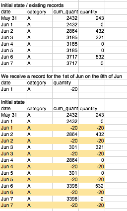
In the example shown above, we receive a record on the 8th of June for the 1st of Jun. Snapshot data is already available until the 7th of Jun. As we cannot update the existing records, we just insert new records (highlighted in yellow) for evert day since the 1st of Jun to correct the existing records. This approach was suggested by Nelson Sousa.
It is worth noting that the Mondrian Cube Definition should easily handle this scenario without requiring any changes, however, the ETL might need some adjustment (e.g. when accumulating snapshot figures get sourced, they have to get aggregated).
An alternative approach
The previously discussed approach was quite difficult to implement - difficult mainly because we had to show the age of a given item in working days (in a given state/event on a given day).
Here is an alternative approach I came up with, which is good for a quick prototype. I wouldn’t use it for production as it generates way too much data - unless you are not worried about this.
Outline of the Strategy

You will notice that we keep on creating negating records and the pairs have +1 and -1 counters (quantity_moving). The difference to the other approaches is that the ETL creates fillers for the days in between the entering and exit record. Notable addition is the quantity_on_hand field, which is set to 1 for every day we actually have this object in the given state/event. Now just put a Mondrian Schema on top, et voilá: you have everything! Mondrian will sum up the quantity_on_hand for a given day, which will give you the accumulative snapshot figures and at the same time you also have access to figures about items entering and exiting a given status (quantity_moving).
Also notice, that for this a particular issue_id we had a raw record for 2015-06-06 and 2015-06-15, but nothing thereafter. There were other records in the source data available last time we imported, so we had to take the maximum date from the source data and generate rows for this issue id up to that date. This will make sure that quantity_on_hand figures are correct for all dates.
Another point to consider is that if an issue id enters and exists a certain state within the same day, we do not want to consider it for quantity_on_hand. The snapshot is taken e.g. at the end of the day, hence intra-day changes are not represented. To detect intra-day changes, the ETL has to generate an age in days field based on which the quantity_on_hands figure can be calculated correctly.
Pros and Cons
Drawbacks of the strategy:
- Data Explosion: We create records for every day for every item in a given state (except closed).
- Snapshot: Once the cumulative sum for a certain combination of dimension reaches 0, no fillers are created (as a normal snapshot would have) (it would still have records for days where there are no facts to report on), but on the other hand side, you do not create empty facts in fact tables either. I do not think this is much of a concern for an end user. The end user will only see a blank report if there are no facts at all or just see data for dimensions where there is a cumulitive sum. However, if you need these fillers, you can create them in an additional ETL process.
Pros:
- It’s very easy to understand - I doubt it get’s any simpler than this.
- It’s very easy to check the results as all calculated/derived fields are generated on the most granular level.
- There is only one output table which provides all required results.
- It should be easy to run this in parallel (partitioning by
issue_ide.g.).
OLAP SCHEMA: When analysing Quantity On Hand exclude the status closed. Status closed is the only status that items never leave. So there is not much use of having a cumulative sum for this status and hence this strategy also does set quantity_on_hand_eod to 0 for status closed records. In general, we are not interested in having a cumulative sum for closed items since the beginning of the service. We are more likely to ask How many issues were closed this week?, which can be answered by using quantity_moving. For all other statuses (which have an in and out movement) we require quantity_on_hand_eod in order to answer the question How many issues are in status X on a given day?. Another advantage of not generating a cumulative sum for status closed is that we do not have to create a huge amount of clones/fillers. We only have to create fillers for all other statuses (which have an in and out movement).