The aim of this tutorial is to present a map with election results. We want to focus on the task at hand - we do not want to reinvent the wheel. This article is particular aimed towards people new to GIS - Geographic Information Systems. We often see the need to display geographic metrics as part of a business dashboard. There is a varying degree of out-of-the-box support for these kind of requirements among business intelligence tools. In some projects, people might go to great lengths to implement this requirement. With this article I want to show that a specific group of people have focused on solving this kind of problem for many years and that there is no need to reinvent the wheel! And you will even be more pleased to here, that most of these tools come for free.
We will start a new project now. All files related to this project can be downloaded from here.
The Map
Initially we will have to acquire the map that we will be working with. Our aim is to create a map of Great Britain displaying the latest election results. A common map file format is a Shapefile. Unlike the name might indicate, it is actually a collection of files, one of them being a shapefile with the map details, a database file including all the features data, a projection file etc.
Let’s understand the basics first:
Shapefile: Shapefiles can store all the commonly used spatial geometries (points, lines, polygons) along with the attributes to describe these features. Unlike other vector formats, a shapefile comes as a set of three or more files – the mandatory .shp, .shx, .dbf and the optional .prj file The .shp file holds the actual geometries, the .shx is an index which allows you to ‘seek’ the features in the shapefile, the .dbf file stores the attributes and the .prj file specifies the projection the geometries are stored in. (Source)
If shapefiles do not sound familiar to you, chances are you really would like to understand what to do with them. If you try opening this kind of file with a text editor, you will realize that this is a binary file type. So we have to find a program/app which can handle shapefiles. There are at least two GIS open source desktop clients which I came across:
We will take a look at QGIS a bit later on. First we will load the shape file into a GIS enabled database: This is not really necessary, but we are ambitious and want to make the best out of it!
Acquiring the Shapefile
The Office of National Statistics website points to this page. Choose Download Products > Boundaries. Here we have the option to download [Boundaries : Westminster_parliamentary_constituencies_(GB)_2013Boundaries_(Full_Extent).zip](https://geoportal.statistics.gov.uk/Docs/Boundaries/Westminster_parliamentary_constituencies(GB)2013_Boundaries(Full_Extent).zip) - but the simplified version will do as well. Actually the simplified version is better, as it we do not require a lot of detail for our map and this map is smaller in size. Unzip the file. If you are already familiar with QGIS, you can already open the shapefile with it and check that the map matches what you are looking for. All the other readers - hold on - we will do this a bit later on.
Understanding the Projection
It is essential to understand which projection the shape file uses. Thankfully most shapefiles include this info. Each shapefile includes a *.prj file:
“If you open up the .prj file from the data directory, you’ll see the projection definition. A common problem for people getting started with PostGIS is figuring out what SRID number to use for their data. All they have is a .prj file. But how do humans translate a .prj file into the correct SRID number? Plug the contents of the .prj file into this online page. This will give you the number (or a list of numbers) that most closely match your projection definition. There aren’t numbers for every map projection in the world, but most common ones are contained within the prj2epsg database of standard numbers.” Source
Acquiring the Data
You can download the UK general election results 2015 election data from here.
The GIS Database
A few databases offer GIS support - one of the most popular is PostgreSQL, for which an extension called PostGIS is available - which we will use. Installing PostGIS is fairly straight forward, so I will not cover it here. For details see this documentation.
Creating the GIS database
Let’s create a dedicated database for our tutorial:
-- for postgresql
CREATE DATABASE elections;

\c elections

CREATE EXTENSION postgis;
-- check correct installation
SELECT postgis_full_version();

CREATE SCHEMA stg;
Import a Shapefile to PostGIS
A shapefile holds all the geographic details - in simple terms, it’s the map we will be working with.
Convert the projection info into standard ESPG codes: To get the correct spatial reference identifier (SRID) put the contents of the .prj file into this online Prj2EPSG converter. It turns out that our shape file has an SRID of 27700 (which is based on the British_National_Grid)
We could import our shape file like this (don’t execute this):
shp2pgsql -c -D -s 27700 -i -I PCON_DEC_2013_GB_BGC.shp stg.uk_map_constituencies > uk_map_constituencies.sql
But ideally we also want to convert it straight away to the required target coordinate system (execute this now):
shp2pgsql -c -s 27700:4326 -i -I PCON_DEC_2013_GB_BGC.shp stg.uk_map_constituencies > uk_map_constituencies.sql
Next let’s execute the generated SQL script:
psql -hlocalhost -delections -Upostgres < uk_map_constituencies.sql
Check with your SQL client that the table exists, e.g.:
SELECT * FROM stg.uk_map_constituencies LIMIT 20;
References:
- Loading Data Into PostGIS
- [Specifications for coordinate reference systems] (http://spatialreference.org/ref/epsg/26918/)
- StackExchange
The GIS Desktop App - Your local GIS Power House
There are various GIS desktop applications available. We will be using the open source QGIS app.
Viewing the Map
Download the most popular open source GIS app QGIS from here. The installation is fairly straight forward, so I will not cover the details here.
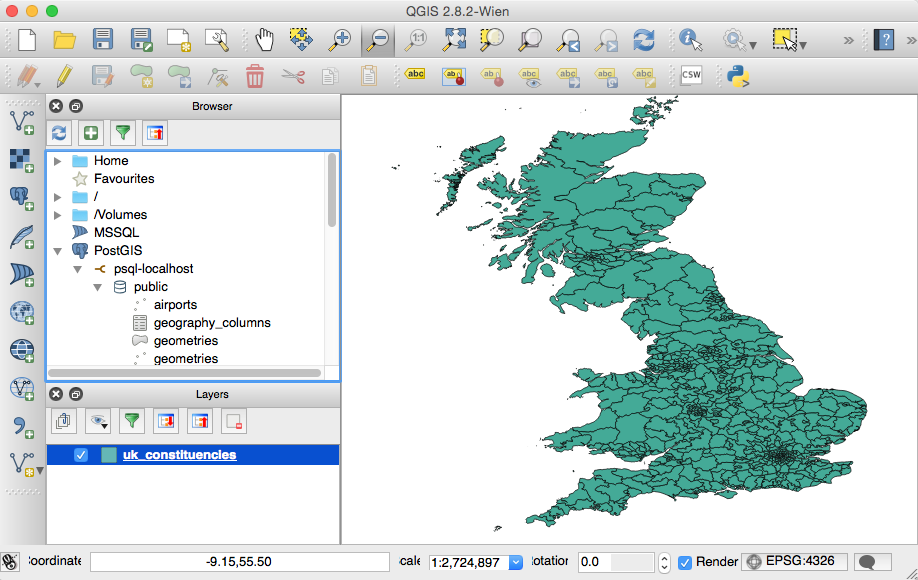
Open the app. In the Browser panel right click on PostGIS and choose New Connection:
Provide the connection details. Once connected, expand the node and double click on our uk_map_constituencies table, which will add it to the Layers panel and herewith display the map in the main window:

I guess you are with me when I am saying that exploring the geo data visually is a far better experience!
The basics of QGIS are quite easy to learn. If you are looking for a good intro book on QGIS, I can recommend Getting started with GIS - Using QGIS (available on Amazon), which provides both an introduction to GIS and QGIS - so this really ideal for beginners.
How to add your data
Our map looks rather uninteresting - let’s add some data: We can find the UK general election data 2015 - collated results (XLS) online here. However, this data requires a bit of cleaning-up as there quite some variations on the party names - so I recommend using the one I provide in the project folder.
Let’s create the required tables now:
CREATE TABLE stg.uk_voting_results
(
  firstname VARCHAR(255)
, lastname VARCHAR(255)
, party_name VARCHAR(255)
, constituency_name VARCHAR(255)
, press_association_number INTEGER
, ons_gss_code VARCHAR(20)
, count_votes INTEGER
)
;

CREATE INDEX uvr_press_association_number
ON stg.uk_voting_results(press_association_number)
;

CREATE TABLE stg.uk_voting_constituencies
(
  press_association_number INTEGER
, constituency_name VARCHAR(255)
, ons_gss_code VARCHAR(20)
, constituency_type VARCHAR(20)
, count_eligible_electors INTEGER
, count_valid_votes INTEGER
)
;

CREATE UNIQUE INDEX uvc_press_association_number
ON stg.uk_voting_constituencies(press_association_number)
;
I created a Pentaho Data Integration transformation to import the data into our database. Run the tr_import_election_data.ktr to populate these two tables. Adjust the file path in the ETL transformation.
Next we have to join all the required data to create a list of election winners by constituency with the geographic feature:
CREATE TABLE stg.uk_voting_winners
AS
SELECT
    constituency_name
    , party_name
    , a.count_votes
    , a.share_votes
    , geom
FROM stg.uk_voting_results a
INNER JOIN
(
    SELECT
        press_association_number
        , MAX(count_votes) AS count_votes
    FROM stg.uk_voting_results
    WHERE
        press_association_number IS NOT NULL
    GROUP BY 1
) b
ON
    a.press_association_number = b.press_association_number
    AND a.count_votes = b.count_votes
INNER JOIN stg.uk_map_constituencies c
ON c.pcon13cd = a.ons_gss_code
;
How to color code the map
In the QGIS Browser panel right click on our previously defined database connection psql-localhost-elections and choose Refresh. The uk_voting_winners table should show up now.

Double click on the uk_voting_winners table and it will be added to the Layers panel. If you have other layers already in there, disable them by unticking the check box next to them.
Right click on the uk_voting_winners Layer and choose Properties:

Make sure the Style section is selected on the very left hand side of the Layer Properties window. Define the following settings:
- At the top change the value in the the drop down menu from Single Symbol to Categorized.
- Choose
party_nameas the Column. - Click the Classify button. This will populate the table above the button with the distinct values of the
party_namecolumn and assign a random color. We could spend more time here and create a custom Color ramp, but I think for now let’s just click the OK button and check the result.

Another point that comes to our attention when looking at the distinct party_name values is that the spelling of the party names is not consistent. We will have to clean this list at some later point.
It’s also worth noting that at the very end of the list you will find the default color: Default in the sense that if a value occurs which does not show up in the list, this color will be assigned.
Your map should look like this now:

We have a color coded map now … this was easy! It’s not a perfect map, but it’s a good start!
If you have some spare time, you can apply the correct list of Color Codes for each political party - see here.
Note: Styles can be exported to standard conform SLD file type. SLD is an acronym for Style Layer Descriptor. This will allow you to reuse the style definition e.g. in map servers like GeoServer or MapServer. Using the properties dialog in QGIS to define all the styling is very convenient and easy - it saves you from writing a long winded XML document. To export a style, simply open the layer’s Properties dialog and click on the Style button at the bottom of the dialog. Then choose Save Style > SLD File.

The content of the SLD file looks like this (partial extract):
<?xml version="1.0" encoding="UTF-8"?>
<StyledLayerDescriptor xmlns="http://www.opengis.net/sld" xmlns:ogc="http://www.opengis.net/ogc" xmlns:xsi="http://www.w3.org/2001/XMLSchema-instance" version="1.1.0" xmlns:xlink="http://www.w3.org/1999/xlink" xsi:schemaLocation="http://www.opengis.net/sld http://schemas.opengis.net/sld/1.1.0/StyledLayerDescriptor.xsd" xmlns:se="http://www.opengis.net/se">
  <NamedLayer>
    <se:Name>uk_voting_winners</se:Name>
    <UserStyle>
      <se:Name>uk_voting_winners</se:Name>
      <se:FeatureTypeStyle>
        <se:Rule>
          <se:Name>Conservative Party</se:Name>
          <se:Description>
            <se:Title>Conservative Party</se:Title>
          </se:Description>
          <ogc:Filter xmlns:ogc="http://www.opengis.net/ogc">
            <ogc:PropertyIsEqualTo>
              <ogc:PropertyName>party_name</ogc:PropertyName>
              <ogc:Literal>Conservative Party</ogc:Literal>
            </ogc:PropertyIsEqualTo>
          </ogc:Filter>
          <se:PolygonSymbolizer>
            <se:Fill>
              <se:SvgParameter name="fill">#a72cdf</se:SvgParameter>
            </se:Fill>
            <se:Stroke>
              <se:SvgParameter name="stroke">#000000</se:SvgParameter>
              <se:SvgParameter name="stroke-width">0.26</se:SvgParameter>
              <se:SvgParameter name="stroke-linejoin">bevel</se:SvgParameter>
            </se:Stroke>
          </se:PolygonSymbolizer>
        </se:Rule>
...
Export the SLD file now - we will use it later on when we configure the map on the server. Also, if you haven’t done so already, save the current QGIS project.
The Map Server - Publishing the Map and Associated Data
The two most popular open source map servers are MapServer and GeoServer. We will take a look at the latter one. These servers can consume standard OGC (Open Geospatial Consortium) web-mapping services (also see Wikipedia entry). The standards documents can be found here.
These map server expose the maps also as standard conform web services:
Setting Up GeoServer
Follow the instruction in the official Documentation.
A good quick starter example: Publishing a PostGIS Table
Once the server is running, you can access the website via this URL. The default username is admin and the default password is geoserver.
Configuring the Map
Once you are logged on, the left hand panel provides various options to set up the map in the Data section. The interface is quite intuitive, so I will only provide a high level overview:

- Create a new Workspace: Name it
elections. - Create a new Store (db connection): Name it
psql-electionsand fill out all the required details. - Create a new Layer: Choose
uk_voting_winnersas the base table. Set at the bare minimum the following config details:- Provide the Declared SRS (if not set).
- In the Bounding Boxes area click on Compute from data and Compute from native bounds.
- On the Publishing tab define the Style (if not set).
Note at the bottom of the Data tab the Feature Type Details section: This shows you how the database columns were mapped (e.g. the type of the column
geomis correctly mapped to typeMultiPolygon). - Create Layer Groups - not required in our case. Only necessary if you want to combine various layers.
-
Preview the map: Click on Layer Preview and search for
elections:uk_voting_winners. Then right click on OpenLayers and choose Open in new window. You will see a grey map now with a zoom option. If you click on one of the constituencies, the features/data of this constituency will be displayed in a table below the map: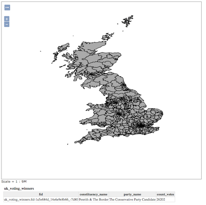
-
Create styles: Finally let’s color code the map. Click on Styles. Click Add new style. Name it
elections, setelectionas Workspace. Leave the Format set to SLD. Click on the Choose File button below Style file (below the huge text box) and choose the SLD style definitions we created earlier on in QGIS. Click Upload. Click on Validate. Finally click on Submit.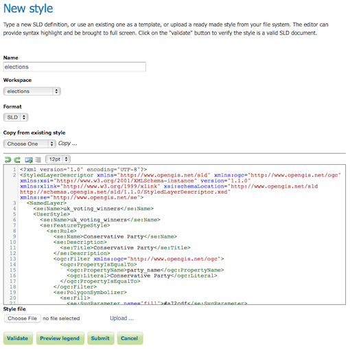
- Go back to the Layers section and search for
uk_voting_winners. Click on the Publishing tab and setelections:electionsas Default Style. Click Save. -
Click on Layer Preview and search for
uk_voting_winners. Click on OpenLayers and a color coded map should be displayed now: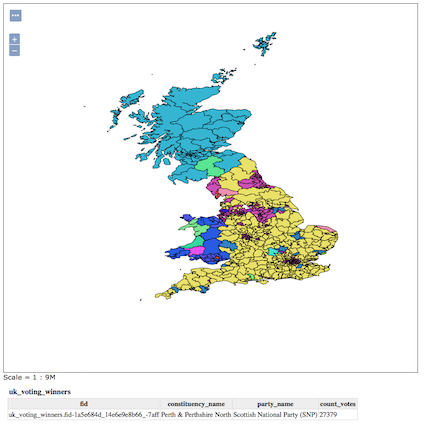
Hurray!!! Our job is done. No coding required! This was certainly a rather simple example, which should have increased your enthusiasm to explore the full feature set of these open source GIS tools. If you are looking for more interactive features for your web maps, take a look at the popular OpenLayers and Leaflet JavaScript frameworks.
Filtering the data and dynamic styles
Just as background info:
How to filter the data on GeoServer:
- SQL Query Parameters: not recommended due to risk of SQL injections. Find an example here.
- FeatureID Filters: See docu
- CQL Filters: See docu
There is also an option to dynamically manipulate the styles defined in the SLD: