In this article we will focus on some advanced data modeling techniques to cover many-to-many and partent-to-child relationships.
Please note that the examples mentioned below can be downloaded from here. To make the most out if it, prepare the following upfront:
- execute the SQL statements
- upload the Mondrian OLAP Schema to Pentaho BI Server or Saiku server
If you are using Pentaho CE BI Server, install either the Saiku CE or Pivot4J Analytics plugin.
Many to Many Hierarchies: Bridge Tables
Usually the relationship between a fact and dimension table in a Kimball style star schema is many to one. However, there are situations where facts can relate to more than one dimensional record.
Example: We are advertising our products online to a particular group of people: Our marketing campaign is targeting people of certain interests. So campaign X could be targeting users, who are interested in sports and entertainment. So how would we model this?
Bridge Tables: This is were bridge tables came in handy: These tables can link one or multiple fact records to one or multiple dimensional records. Bridget tables are also sometimes referred to as helper tables.
The structure of a bridge table looks like this (simplified):
| group key | item key | weight factor |
|---|---|---|
| 1 | 5 | 0.5 |
| 1 | 65 | 0.5 |
| 2 | 3 | 0.333 |
| 2 | 234 | 0.333 |
| 2 | 334 | 0.333 |
The dimensional table looks like this (simplified)
| item key | item name |
|---|---|
| 3 | CC |
| 5 | AA |
| 65 | ZZ |
| 234 | LL |
| 334 | UU |
And the fact table looks like this (simplified):
| date key | group key | measure |
|---|---|---|
| 20141223 | 1 | 235323 |
| 20141223 | 2 | 534213 |
So in the fact table above, the first row links to group 1 in the bridge table, which in turn links to items 5 and 65 in the dimension table. The bridge table also shows a weight factor of 0.5 (so 50%), because we are dealing with two items.
So what’s the difference between a snowflake schema approach and the bridge table?
A snowflake schema is basically about denormalizing a standard dimension and you do not end up having one to many relationships (and hence there is no weighting factor).
Many-to-many or one-to-many?
What kind of relationship does the bridge table cover? Is it many fact records to many dimensional records or one fact record to many dimensional records? Well, there is no hard written rule for this, it depends on the scenario. In some situations you might be able to reuse existing groups (as in our example interest groups) and this will allow you the keep the table size small (many-to-many relationship). However, there are situations were you might have to create a group for each record in the fact table (one-to-many relationship), in which case it could evolve into a slowly changing dimension type 2. (see page 265 DWH Toolkit). Note: A bridge table does not always sit between a fact table and a dimensional table. It is also possible that it sits between two dimensional tables. In example a patient dimension can be linked to a diagnoses group bridge table and this one to a diagnosis dimension. This is also an example where the bridge table could serve as a SCD Type 2 and each group could be unique to one patient.
How to expose your data to the OLAP Cube
To deal with many to many or one to many relationships we set up a bridge table. To make this data structure accessible to an OLAP Cube engine, in example Mondrian (which we focus on here), you will have to create a view, which joins the fact and bridge table and hence exposes it as one “table” to Mondrian.
There are two approaches on how to create this view:
When to use weighting factor
In most cases you will want to multiply the measures with the weighting factor in order to still have correct roll-ups in your cube.
CREATE VIEW tutorial.vw_fact_campaign_funnel AS
SELECT
    f.date_tk
    , f.campaign_name
    , b.interest_tk
    , f.impressions * b.weight_factor AS impressions
    , f.clicks * b.weight_factor AS clicks
    , f.items_bought  * b.weight_factor AS items_bought
    , f.basket_value * b.weight_factor AS basket_value
FROM tutorial.fact_campaign_funnel f
INNER JOIN tutorial.bridge_interest_group b
    ON f.interest_group_tk = b.interest_group_tk
;
In some cases, however, you might want to have an Impact Report: For each dimensional value you want to see the sum of all measures (without using any weighting factor). In our example you possibily would like to understand which particular interest generated most revenue. The SQL for the view would look like this:
CREATE VIEW tutorial.vw_fact_campaign_funnel_impact AS
SELECT
    f.date_tk
    , f.campaign_name
    , b.interest_tk
    , f.impressions
    , f.clicks
    , f.items_bought
    , f.basket_value
FROM tutorial.fact_campaign_funnel f
INNER JOIN tutorial.bridge_interest_group b
    ON f.interest_group_tk = b.interest_group_tk
;
How to populate the bridge table
I won’t go into much detail here: You can either use your ETL tool to populate the bridge table or a stored procedure.
Using Pentaho Kettle you could generate a process like this one:
Main job:

Transformation to maintain the dimension:

Transformation to check if group exists:

Here we just use a SQL statement to perform the check:
SELECT
    interest_group_tk
FROM
(
    SELECT
        b.interest_group_tk
        , CASE
            WHEN COUNT(b.interest_tk) = ${VAR_INTERESTS_COUNT} THEN 1
            ELSE 0
         END AS group_found
    FROM tutorial.bridge_interest_group b
    WHERE
        interest_tk IN ( ${VAR_INTEREST_TKS_LIST} )
    GROUP BY 1
    ORDER BY 1
) AS group_search
WHERE
    group_found = 1
Transformation to maintain the bridge table:

How to create the OLAP Cube definition
The OLAP Schema for Cube, which uses a bridge table, would look like this:
<Cube name="Campaign Funnel" visible="true" cache="true" enabled="true">
    <Table name="vw_fact_campaign_funnel" schema="tutorial"/>
    <DimensionUsage source="Date" name="Date" caption="Date" visible="true" foreignKey="date_tk"/>
    <Dimension name="Campaign" type="StandardDimension" visible="true" highCardinality="false">
        <Hierarchy name="Campaign" visible="true" hasAll="true" allMemberName="Total" allMemberCaption="Total">
            <Level name="Campaign" column="campaign_name" visible="true" type="String" levelType="Regular"/>
        </Hierarchy>
    </Dimension>
    <Dimension name="Interest" foreignKey="interest_tk" type="StandardDimension" visible="true" highCardinality="false">
        <Hierarchy name="Interest" primaryKey="interest_tk" visible="true" hasAll="true" allMemberName="Total" allMemberCaption="Total">
            <Table name="dim_interest" schema="tutorial"/>
            <Level name="Interest" column="interest" visible="true" type="String" levelType="Regular"/>
        </Hierarchy>
    </Dimension>
    <Measure name="Impressions" column="impressions" datatype="Numeric" formatString="#,##0.00" aggregator="sum"/>
    <Measure name="Clicks" column="clicks" datatype="Numeric" formatString="#,##0.00" aggregator="sum"/>
    <Measure name="Items in Basket" column="items_bought" datatype="Numeric" formatString="#,##0.00" aggregator="sum"/>
    <Measure name="Basket Value" column="basket_value" datatype="Numeric" formatString="#,##0.00" aggregator="sum"/>
</Cube>
<Cube name="Campaign Funnel Impact" visible="true" cache="true" enabled="true">
    <Table name="vw_fact_campaign_funnel_impact" schema="tutorial"/>
    <DimensionUsage source="Date" name="Date" caption="Date" visible="true" foreignKey="date_tk"/>
    <Dimension name="Campaign" type="StandardDimension" visible="true" highCardinality="false">
        <Hierarchy name="Campaign" visible="true" hasAll="true" allMemberName="Total" allMemberCaption="Total">
            <Level name="Campaign" column="campaign_name" visible="true" type="String" levelType="Regular"/>
        </Hierarchy>
    </Dimension>
    <Dimension name="Interest" foreignKey="interest_tk" type="StandardDimension" visible="true" highCardinality="false">
        <Hierarchy name="Interest" primaryKey="interest_tk" visible="true" hasAll="true" allMemberName="Total" allMemberCaption="Total">
            <Table name="dim_interest" schema="tutorial"/>
            <Level name="Interest" column="interest" visible="true" type="String" levelType="Regular"/>
        </Hierarchy>
    </Dimension>
    <Measure name="Impressions" column="impressions" datatype="Numeric" formatString="#,##0.00" aggregator="sum"/>
    <Measure name="Clicks" column="clicks" datatype="Numeric" formatString="#,##0.00" aggregator="sum"/>
    <Measure name="Items in Basket" column="items_bought" datatype="Numeric" formatString="#,##0.00" aggregator="sum"/>
    <Measure name="Basket Value" column="basket_value" datatype="Numeric" formatString="#,##0.00" aggregator="sum"/>
</Cube>
Parent-Child Hierarchies
Parent-child are sometimes called variable depth hierarchies as well. Typically a organizational personal structure is modeled as a parent-child hierarchy.
To represent a parent-child hierarchy we initially only have to create one table, which lists the employee and their supervisor.
In the dimensional records below we can see that Eric reports into Bill and then Frank:
| supervisor_id | employee_id | full_name |
|---|---|---|
| null | 1 | Frank |
| 1 | 2 | Bill |
| 2 | 3 | Eric |
This table is sufficient for Mondrian, but the performance will not be very good. In order to query these hierarchies efficiently with SQL we need a Closure Table.
In the closure table we would have following records for Eric:
| supervisor_id | employee_id | distance |
|---|---|---|
| 1 | 3 | 2 |
| 2 | 3 | 1 |
| 3 | 3 | 0 |
As you can see the last record means Eric reports into himself and the distance is 0. The next record further up tells us that Eric reports into Bill and the distance is 1 (meaning on level up). Finally we also see that Eric reports into Frank, who is two levels up the hierachy (distance: 2).
In the scenario depicted here, the closure table would also need similar records for Bill and Mark, showing all their relationships and distances to themselves and anyone above them in the hierarchy.
Closure Table: A closure table includes a record for each member and ancestor relationship (regardless of depth). It contains an additional column which shows the distance (number of levels) between the specific level and the ancestor. In example: Frank reports into Mark, so the distance is 1. Another important aspect to remember about the closure table is that its use is optional: You can still directly join the fact with the dimensional table without using the closure table.
How to populate the closure table
You can either use a SQL statement like this (PostgreSQL):
TRUNCATE tutorial.item_closure;
INSERT INTO tutorial.item_closure
WITH RECURSIVE q AS (
    SELECT
        item_tk
        , item_tk AS closure_parent_tk
        , item_parent_tk
        , item_name
    FROM tutorial.dim_item
    UNION ALL
    SELECT
        q.item_tk
        , p.item_tk AS closure_parent_tk
        , p.item_parent_tk
        , p.item_name
    FROM tutorial.dim_item AS p
    INNER JOIN q
        ON p.item_tk = q.item_parent_tk
)
SELECT
    item_tk
    , closure_parent_tk
FROM q
;
For Oracle it looks something like this:
INSERT INTO tutorial.item_closure
SELECT i.id
     , connect_by_root i.id AS parent_id
  FROM item i
 CONNECT BY PRIOR i.id = i.parent_id
;
Or alternatively you can just use the Closure step in Pentaho Kettle to populate the closure table.
How to create the OLAP Cube definiation
The Mondrain cube definition for a parent-child hierarchy with a closure table would look like this:
<Cube name="Sales" visible="true" cache="true" enabled="true">
    <Table name="fact_sales" schema="tutorial"/>
    <DimensionUsage source="Date" name="Date" caption="Date" visible="true" foreignKey="date_tk"/>
    <Dimension name="Employees" foreignKey="employee_tk">
        <Hierarchy hasAll="true" allMemberName="Total" primaryKey="employee_tk">
            <Table name="dim_employee" schema="tutorial"/>
            <Level name="Employee" uniqueMembers="true" type="String"
            column="employee_tk" nameColumn="full_name" parentColumn="supervisor_tk" nullParentValue="0">
                <Closure parentColumn="supervisor_tk" childColumn="employee_tk">
                    <Table name="employee_closure" schema="tutorial"/>
                </Closure>
            </Level>
        </Hierarchy>
    </Dimension>
    <Measure name="Sales" column="sales" datatype="Numeric" formatString="#,##0.00" aggregator="sum"/>
</Cube>
Notes on the standard parent-child dimension (not closure table) Mondrian schema declartion:
- In your dim table make sure that the root elements show a
NULLvalue for the parent. Alternatively specify thenullParentValueproperty. - Also make sure that
uniqueMembersis set totrue- this is a main requirement of parent-child hierarchies.
If you downloaded the same files and set up everything, run this MDX query in your favourite client:
SELECT
	([Measures].[Sales])
	ON COLUMNS,
	[Employees].AllMembers ON ROWS
FROM [Sales]
Note: Saiku Analytics currently doesn’t seem to support hierarchical dimensions in the drag and drop interface properly. However, running the above MDX query will show the correct results: Just click on the Switch to MDX Mode icon and copy and paste the above query there.
How to show measures for member only
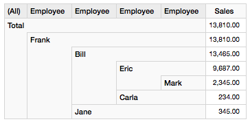
Once you start using a parent-child hierarchy, the measures get all rolled up, meaning that sales of managers will include their own sales as weel as the sales of all their employees. However, it is still possible to show only the managers (and other’s) personal salary by using the MDX property DataMember:
WITH MEMBER [Measures].[Personal Sales] AS
	([Employees].DataMember, [Measures].[Sales])
SELECT
	{[Measures].[Sales], [Measures].[Personal Sales]}
	ON COLUMNS,
	[Employees].AllMembers ON ROWS
FROM [Sales]
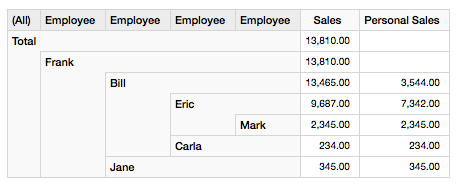
Note how Frank’s sales are made up of Bill’s and Jane’s team’s sales. The figure includes Frank’s personal sales as well - but in this case it is not relevant as Frank seems to have been generating no sales at all.
Bill’s sales are made up of his own sales, Eric’s team’s sales and Carla’s sales:
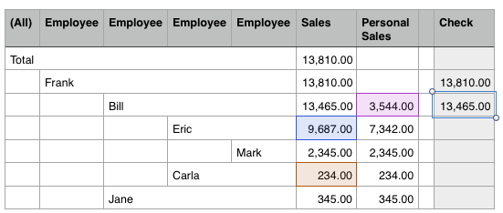
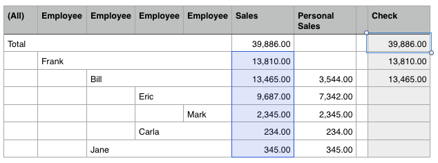
The Total (AllMember) sales is just the same as Frank’s sales - as you would expect.
Let’s see what Mondrian is doing under the hood, when we trigger this MDX query:
-- sourcing fact records
-- note join on closure table
select
	"employee_closure"."supervisor_tk" as "c0" 	, sum("fact_sales"."sales") as "m0"
from
	"tutorial"."employee_closure" as "employee_closure"
	, "tutorial"."fact_sales" as "fact_sales"
where
	"fact_sales"."employee_tk" = "employee_closure"."employee_tk"
group by
	"employee_closure"."supervisor_tk"


-- finding the child of a specific member
select
	"dim_employee"."employee_tk" as "c0"
	, "dim_employee"."full_name" as "c1"
from "tutorial"."dim_employee" as "dim_employee"
where
	"dim_employee"."supervisor_tk" = '1'
group by
	"dim_employee"."employee_tk", "dim_employee"."full_name"
order by
	"dim_employee"."employee_tk" ASC NULLS LAST

select
	"dim_employee"."employee_tk" as "c0"
	, "dim_employee"."full_name" as "c1"
from "tutorial"."dim_employee" as "dim_employee"
where
	"dim_employee"."supervisor_tk" = '2'
group by
	"dim_employee"."employee_tk", "dim_employee"."full_name"
order by
	"dim_employee"."employee_tk" ASC NULLS LAST

-- ... and so forth ... scanning all records
Questions
The figure for the AllMember looks seriously wrong!
I tested the above example first with the Saiku Analytics plugin, which at the time of this writing ships with mondrian-3.6.7.jar. The amount of sales for the AllMember was wrong - it was the sum of all the roll-ups, when it should have been just the same as Frank’s sales amount. However, when testing the example with mondrian-3.8.0.0-209.jar, which ships with biserver-ce v5.2, the totals are correct.
Does Mondrian use the distance field?
It doesn’t seem to be required, as it just works without it. And even if it is available, Mondrian doesn’t seem to be using it. The online docu states: “The distance column is not strictly required, but it makes it easier to populate the table”.
Another Example
Previously we were looking at an organizational hierarchy, where usually one person is the big boss - the top level parent. However, there are other use cases where that can be serveral top evel parents, in example a category hierarchy like the one dipicted in the Parent/child dimensions in Jasper Analysis blog post: This is a very interesting example indeed!
WITH MEMBER [Measures].[Member Expenses] AS
    ([Measures].[Expenses], [Item].DataMember)
SELECT
    {[Measures].[Expenses], [Measures].[Member Expenses]} ON COLUMNS
    , [Item].AllMembers ON ROWS
FROM [Item Expenses]
And the result looks like this (just without the Check column):

On first inspection the figure for Fowl might look a bit weird, but we have to keep in mind here that the fact table contains records on Chicken (which is one level below) as well as Fowl level. So in this case 56.90 for Chicken and 48.00 for Fowl gets summed up, hence our OLAP Client displays the figure 104.90 for Fowl.
Watch the video below to see this sample in action using Pentaho biserver-ce with the Pivot4J Analytics plugin:
Ragged Hierarchies
Ragged hierachies are similar to standard hierarchies, just that levels can be skipped. In example not every country has states. In this case a city’s parent is the country and in the UI, the state level should not be shown. Entries for states still have to exist though in the dimensional table, however they will have no value. You can use the Mondrian hideMemberIf level attribute and set its value to ifBlankName. The member will not appear then in UI if it is NULL, blank or all whitespace. (Note there are other options as well, so Mondrian doc).
Sources
- Mondrian Documentation
- Mondrian in Action
- The Data Warehouse Toolkit, Ralph Kimball and Margy Ross
- Parent/child dimensions in Jasper Analysis
- Data Warehouse Structures: a bridge-table