How to implement stream partitioning
In this section we will focus on partitioning, which is a special case of using multiple copies of one step.
Take this rather simple transformation (which you can download from here):
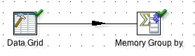
We used a Data Grid step to define some dummy data:
| fruit | quantity |
|---|---|
| bananas | 3 |
| bananas | 234 |
| bananas | 463 |
| bananas | 36 |
| apples | 3466 |
| apples | 243 |
| grapes | 436 |
| grapes | 234 |
| grapes | 457 |
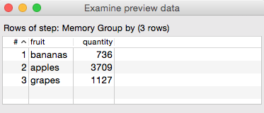
Then we added a Memory Group by step to sum up the quantity by fruit. If we run this transformation, we get following result:
| fruit | quantity |
|---|---|
| apples | 3709 |
| grapes | 1127 |
| bananas | 736 |
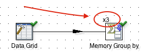
Now let’s imagine we are dealing with a huge input dataset and we can leverage the power of a multicore machine: The first idea that comes to mind is running multiple copies of the Memory Group by step in parallel. Right click on the Memory Group by step and choose Change number of copies to start: Set it to 3 e.g.. Notice that on the top left hand side of the step icon we can see x3 now - indicating that 3 copies of this step will be run:
Before we are too content with ourselves, let’s check the results to see if everything is still as expected:
| fruit | quantity |
|---|---|
| grapes | 436 |
| bananas | 39 |
| apples | 243 |
| grapes | 457 |
| bananas | 463 |
| apples | 3466 |
| grapes | 234 |
| bananas | 234 |
Now this looks rather strange! Why do we get a totally different result you might ask? The answer to this question is that we are sending records in a round-robin (random) fashion to 3 separate copies of the Memory Group by step. Each of these copies of this step does their own processing: So each one sorts and aggregates and the result we see above is just a union of the 3 resultsets generated by the 3 copies.
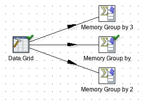
In a nutshell, creating 3 copies of a given step is just like having 3 steps of the same type and the incoming hops have the data-movement set to Distribute (round-robin):
Parallelism in PDI is an interesting concept, but it’s not really helping us in this case (Note we are looking at quite a special case here as we are using the Memory Group by step), unless - of course - there is some way to ensure that keys of the same value go to the same copy of our Memory Group by step! Now that’s a genius idea isn’t it? So if we send all the apples records to one copy, then all of them get aggregated there and the union of all step copies’ resultsets would show one entry for apples with the correct sum.
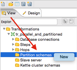
So what we effectively want to do is partition our data. Thankfully Pentaho Data Integration allows us to generate one or more Partition Schemas in the View panel.
In the View panel, right click on Partition schemas and choose New:
The Partitioning Schema Dialog allows us to define the following properties:
| Partitioner Type | Environment | Description |
|---|---|---|
| dynamic partitioner | Cluster | PDI automatically partitions the data that is sent to the slave servers based on the number of slave servers, making sure that records with certain key values are grouped together and are sent to the same slave server. E.g. We want all records with fruit name ‘apples’ to be part of one particular partition and hence go to one particular slave server. |
| number of partitions | Cluster | This is similar to Numbers of copies which you can define in a non-partitioned setup by right clicking on a step. |
| partition names | Single machine | define a static list of partition names - this can be any name |
Note: For a clustered environment you have to set the first two options and for a single machine setup the last option only.
For our example we define 3 partitions by listing the partition names, which can be any names - they do not bear any meaning:
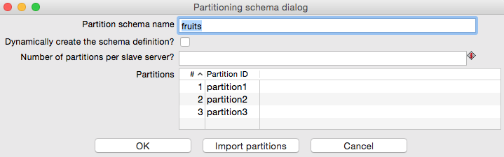
Note: Using a static value for the number of partitions isn’t really a good approach. Set up a parameter for the partition number.
Note: Currently there is no way to define the number of partitions for single machine execution (as opposed to defining the names). I created a Jira case for this.
Right click on the Memory Group by step and choose Partitioning. Now you will be asked for the Partitioning Method:
- None: This option does not use any partitioning schema, but whatever data-movement option is defined for the input hops (Copy or Round-robin).
- Mirror to all partitions: This relates to database partitions only (partitions in the sense that there is one database and several replicas [1:1 copies, sharing], each one being treated as a database (NOT table) partition), allows to persist the same data to mulitple database partitions.
- Remainder of division: This is the standard partitioning method: Kettle divides the partitioning field by the number of partitions. In the case that the partitioning fields has another data type than integer, a checksum is used.
So in our case we want to use Remainder of division as the Partitioning Method. Next you can define the Partitioning Schema to use - select the one just created. And finally you can define the partitioning key (Mod partitioner): Choose fruit.
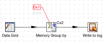
Our choice will be indicated on the canvas, note the Dx3 and fruits labels next to the Memory Group by step:
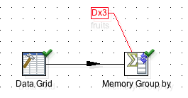
Important: Did you notice that the indicator for number of copies disappeared? Remember before we saw a
x3indicator just above the Memory Group by step. The reason for this is that the partitioning schema automatically creates the required number of copies of a particular step. Each partition will be send to one step copy.
Let’s run the transformation now and see if the result is correct:
| fruit | quantity |
|---|---|
| apples | 3709 |
| grapes | 1127 |
| bananas | 736 |
This time the result is correct. The added benefit is that our transformation should process the data a lot faster now.
Caution with Previewing the data
Since PDI version 5 we have a fancy new Preview data tab available. This is a very handy utility as it allows you to click on any step of the transformation to see how the processed data looks like (you have to execute the transformation first). This is a considerable improvement over the standard Preview step context option.
However, when using a Partitioning Schema the Preview data tab will only show the data of the first copy of a step whereas the step specific Preview context option will show the data of all copies! This can be rather confusing.
When I executed my sample transformation in PDI v5.3, I could see in the Step Metrics tab the 3 copies of the Memory Group by step:
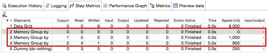
Notice that the first copy didn’t process any rows. When I inspected the Preview data tab I didn’t see any data at all:
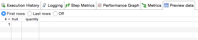
So my first impression was that something had gone totally wrong.
However, when I right clicked on the Memory Group by step and chose Preview, I could see the full resultset:
My conclusion is that the Preview data tab seems to display the data of the first copy of a given step only (at least when using a Partitioning Schema).
A simple workaround for our transformation would be to add a dummy step at the end, for which the Preview data tab would display all the data again.
Scaling out: Clustering
As we are expecting an intense workload, we decide to scale out by using PDI’s clustering feature, which allows you to run an ETL process on several machines. For the purpose of this tutorial we will simulate this by starting the Carte servers locally.
Navigate to the PDI root directory. Let’s start three local Carte instances for testing (Make sure these ports are not in use beforehand):
sh carte.sh localhost 9090
sh carte.sh localhost 9091
sh carte.sh localhost 9092
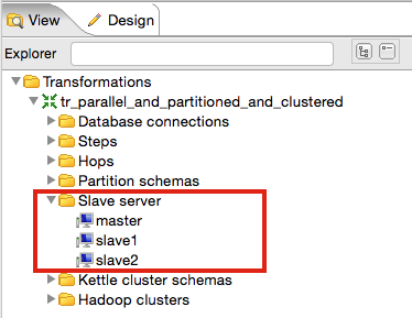
In PDI Spoon click on the View tab on the left hand side and right click on Slave server and choose New. Add the Carte servers we started earlier on one by one and define one as the slave server. Note the default Carte user is cluster and the default password is cluster. Your setup should look like this now:
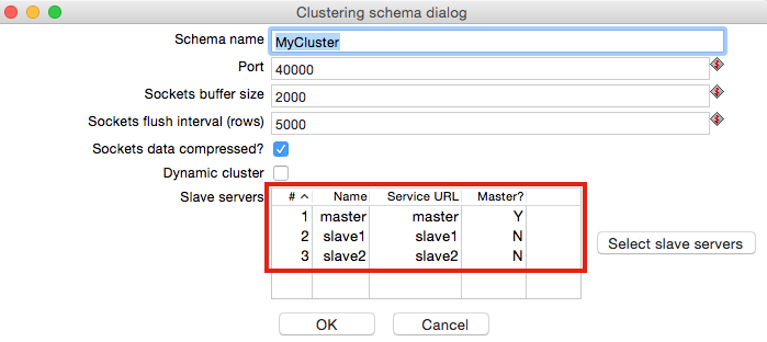
Next right click on Kettle cluster schemas and choose New. Provide a Schema name and then click on Select slave servers. Mark all of them in the pop-up window and select OK.
Next we want to make sure that Kettle can connect to all of the Carte servers. Right click on the cluster schema you just created and choose Monitor all slave servers:
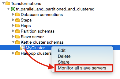
For each of the servers Spoon will open a monitoring tab. Check the log in each monitoring window for error messages.
If all that went well, go to Partition Schemas and change the settings of our previously defined schema: Remove all the partition names and then tick Dynamically create the schema definion and set the number of partitions per slave to 1.
Next right click on the Memory Group by step and choose Clusterings. Choose the cluster you just defined. The transformation should look like this now (You can also download the transformation from download from here):
Notice the Cx2 indicator next to the Memory Group by step. The partitioning indicator also changed to Dx1.
Let’s run the transformation now to see if the results are still the same. Click on the Slave server: master tab and highlight the transformation (you might have to click the Refresh button at the bottom to see it). In the log output you should see something like this:
2015/04/28 19:40:48 - Write to log.0 - ------------> Linenr 0------------------------------
2015/04/28 19:40:48 - Write to log.0 - === FINAL RESULTSET ===
2015/04/28 19:40:48 - Write to log.0 -
2015/04/28 19:40:48 - Write to log.0 - fruit = apples
2015/04/28 19:40:48 - Write to log.0 - quantity = 3709
2015/04/28 19:40:48 - Write to log.0 -
2015/04/28 19:40:48 - Write to log.0 - ====================
2015/04/28 19:40:48 - Write to log.0 -
2015/04/28 19:40:48 - Write to log.0 - ------------> Linenr -1------------------------------
2015/04/28 19:40:48 - Write to log.0 - === FINAL RESULTSET ===
2015/04/28 19:40:48 - Write to log.0 -
2015/04/28 19:40:48 - Write to log.0 - fruit = grapes
2015/04/28 19:40:48 - Write to log.0 - quantity = 1127
2015/04/28 19:40:48 - Write to log.0 -
2015/04/28 19:40:48 - Write to log.0 - ====================
2015/04/28 19:40:48 - Write to log.0 -
2015/04/28 19:40:48 - Write to log.0 - ------------> Linenr 0------------------------------
2015/04/28 19:40:48 - Write to log.0 - === FINAL RESULTSET ===
2015/04/28 19:40:48 - Write to log.0 -
2015/04/28 19:40:48 - Write to log.0 - fruit = bananas
2015/04/28 19:40:48 - Write to log.0 - quantity = 736
2015/04/28 19:40:48 - Write to log.0 -
2015/04/28 19:40:48 - Write to log.0 - ====================
2015/04/28 19:40:48 - Write to log.0 - Finished processing (I=3, O=0, R=0, W=3, U=0, E=0)
This indicates that our transformation works just fine in clustered mode! Here the difference is that the partitioning schema (in our case) is applied to the way the data is sent to the slaves. The first step (Data Grid) and last step (Write to log) execute on the master node, whereas the Memory Group by step (or more precisely the steps copies) run(s) on the slaves.
Combining Data Partitioning for Salves and for Step copies
So there are at least two use cases for partitioning:
- partition the data which flows to copies of a step (let’s think of a non-clustered transformation or parts of the transformation that run on a slave server). E.g. We want all records with fruit name ‘apples’ to go to one partition which in turn goes to one step copy.
- partition the data that is sent to the slave servers, making sure that each slave server gets a specific chunk of the data. E.g. We want all records with fruit name ‘apples’ to go to into one particular partition which then goes to one particular slave.
Note: Combinations of the above are not possible with one Partition Schema. This is because only one partitioning process can run at a time (in our previous example: partition the data for the slaves. If the number of copies to start on slaves is higher than 1, Kettle would have to add a second partitioning process for the step copies). For partitioning data for slave servers we have to set the number of copies always to 1. Any step after this can have more copies.
The example shown below has two partitioning schemas defined: The important point is that the first step that runs on the cluster (Add constants) has only one copy defined, whereas the following one has two copies defined:
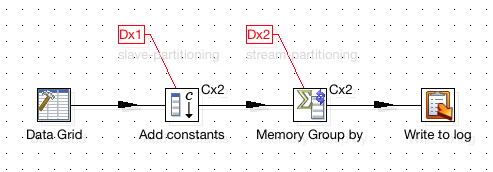
You can also download the transformation from download from here.
To summarise the partition methods for this last example:
- We partition the data which gets sent to the slaves.
- We partition the data which gets sent to the step copies.
Understanding a Clustered Transformation
While at design time we are only dealing with one transformation, once PDI executes the transformation it creates several other transformations behind the scenes:
- Transformation for the master
- Transformations for the slaves
Spoon comes with quite a handy feature, which allows you to visualise this process. In the Execute a transformation just tick Show transformations:
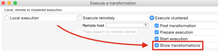
Once you execute the transformation, additional tabs will show up in Spoon showing the generated transformations.
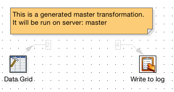
The screenshot below shows the transformation for the master. Note that the grey figures indicate the number of input and output streams:
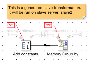
And this is one of the transformations which will run on one of the slave servers:
Going Further
Did you know you can write your own partitioning method for PDI? There is a dedicated Wiki article available with a few examples, which are really worth reading through.
You might also be interest in hearing that the Carte configuration can be specified via an XML file - see here for details.
As you can see, Pentaho Data Integration has an abundance of features - an exciting world ready to be explored!
Sources: