D3 Maps
My previous article Geo Data - The fast lane to publishing a Map provided a very basic introduction to the exciting world of GIS. Again, I’d like to emphasise that the main intention of my GIS articles is to present these maps as part of business dashboards. With this article I want to kick off a short series of articles focused on building maps with the D3 JavaScript framework. D3 is an abbreviation for Data Driven Documents and I strongly suggest that you take a look at the examples provided on the project’s website to get a good understanding of D3’s features.
The series of articles will be based around a single project: We want to present the UK General Election Results 2015 with the help of a map (as has been done quite impressively by BBC).
We will start a new project now. All files related to this project can be downloaded from here.
Considerations
We want:
- a map which loads fast (vector map)
- map data to be stored on the server (instead of being dependent on an external service like Google Maps etc). This is often a requirement when working with confidential data where access to the outside world is locked down.
Basics
The Shapefile
Shapefile: Shapefiles can store all the commonly used spatial geometries (points, lines, polygons) along with the attributes to describe these features. Unlike other vector formats, a shapefile comes as a set of three or more files – the mandatory .shp, .shx, .dbf and the optional .prj file The .shp file holds the actual geometries, the .shx is an index which allows you to ‘seek’ the features in the shapefile, the .dbf file stores the attributes and the .prj file specifies the projection the geometries are stored in. (Source)
If shapefiles do not sound familiar to you, chances are you really would like to understand what to do with them. If you try opening this kind of file with a text editor, you will realize that this is a binary file type. So we have to find a program/app which can handle shapefiles. There are two GIS open source projects which I came across:
Understanding the Projection
It is essential to understand which projection the shape file uses. Thankfully most shapefiles include this info. Each shapefile includes a *.prj file:
“If you open up the .prj file from the data directory, you’ll see the same projection definition. A common problem for people getting started with PostGIS is figuring out what SRID number to use for their data. All they have is a .prj file. But how do humans translate a .prj file into the correct SRID number? Plug the contents of the .prj file into this online page. This will give you the number (or a list of numbers) that most closely match your projection definition. There aren’t numbers for every map projection in the world, but most common ones are contained within the prj2epsg database of standard numbers.” Source
Initial Setup
To follow this tutorial, you will have to make sure you have the following software packages installed. I will not go through the install procedure as I feel there is enough coverage on the internet on this already.
Install GDAL: Download your OS specific version from here.
Note: On Federa execute
sudo yum install gdal.x86_64. On Mac OS X you can use Homebrew to install GDAL:brew install gdal
Install NodeJS.
Install TopoJSON via the Node Package Manager:
$ sudo npm install -g topojson
Verify installation:
$ which ogr2ogr
/usr/local/bin/ogr2ogr
$ which topojson
/usr/local/bin/topojson
We will be using QGIS to visualise the map. Pay attention to the install instructions. On Fedora, all I had to do was to install the client tools like so:
$ sudo yum update
$ sudo yum install qgis qgis-python
Working with Shapefiles
On the Command Line
In this section you will learn how to:
- extract specific map details from a shapefile
- merge shapefiles and
- convert shapefiles to GeoJSON and finally to TopoJSON.
TopoJSON (developed by Mike Bostock) allows us to minify GeoJSON files. Note that this section slightly follows Mike Bostock’s tutorial Let’s Make a Map, which I strongly suggest to have a look at.
Download these files:
Extract these zip files and then run the commands inside the extracted folders (otherwise you will get an error):
Run the next command inside the ne_10m_admin_0_map_subunits folder to extract the country shapes for Great Britain and Ireland:
ogr2ogr
  -f GeoJSON \
  -where "ADM0_A3 IN ('GBR', 'IRL')" \
  subunits.json \
  ne_10m_admin_0_map_subunits.shp
Run the next command inside the ne_10m_populated_places folder to extract the major cities:
ogr2ogr \
  -f GeoJSON \
  -where "ISO_A2 = 'GB' AND SCALERANK < 8" \
  places.json \
  ne_10m_populated_places.shp
Copy both output files (subunits.json and places.json) into a dedicated directory and merge them with following command:
topojson \
  -o uk.json \
  --id-property SU_A3 \
  --properties name=NAME \
  -- \
  subunits.json \
  places.json
Using a GIS client tool
As an alternative to using command line tools you can manipulate maps in a GIS client app.
The QGIS Desktop app will allow us to visualise the shapefile and manipulate it using the GUI, which provides instant feedback - in a nutshell: It will allow spatial geo newbies as well as professionals to work more efficiently.
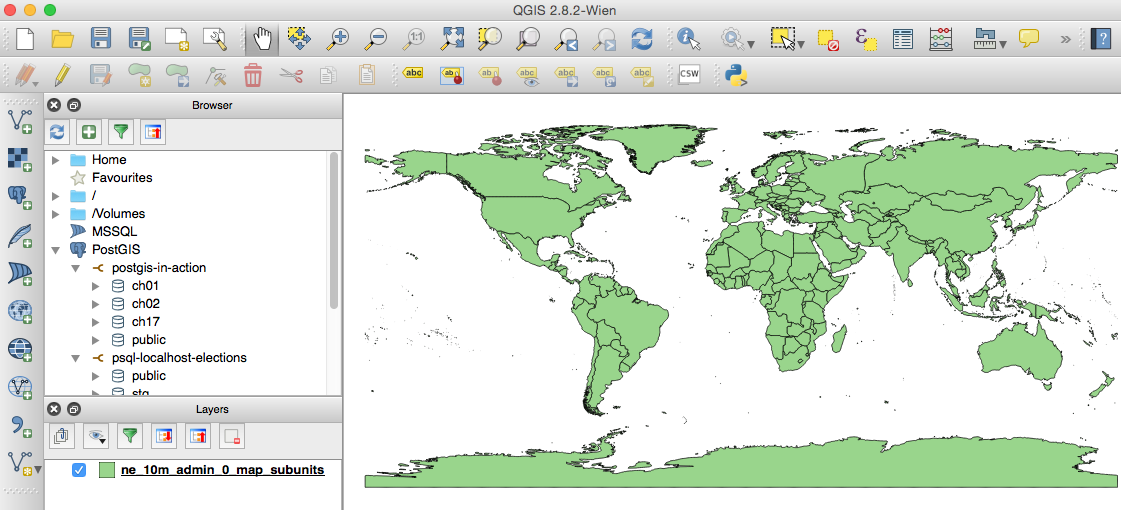
Open the QGIS Desktop app.
On the very left hand side you have various icons with a plus symbol. Click on the Add Vector Layer and click on Browse to add the ne_10m_admin_0_map_subunits/ne_10m_admin_0_map_subunits.shp file. Finally click OK.
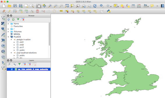
Right click on our map layer and choose Filter. In the Query Builder look for ADM0_A3 from Fields and double click on it, which will populate the Filter expression box at the bottom. Complete the expression so that it looks like the one shown below:
"ADM0_A3" IN ('GBR', 'IRL')
Click OK and the map should show only the UK and Ireland now, but quite likely it will be very small. Click on the Zoom Full button and then you should see the UK and Ireland better:
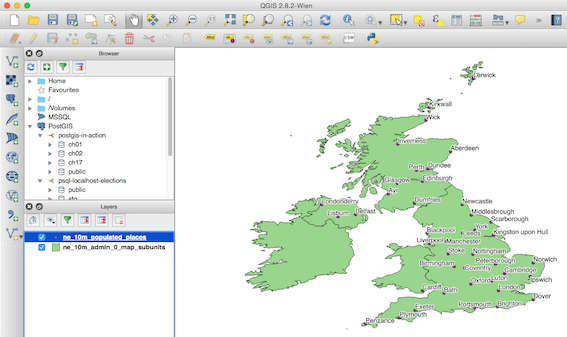
Next click on the Add Vector Layer and choose the ne_10m_populated_places/ne_10m_populated_places.shp shape file. In the Layers panel right click on the populated places layer and choose Filter. Set the expression to:
ISO_A2 = 'GB' AND SCALERANK < 8
We can also add some labels if we wanted to: Right click on the populated places layer and choose Properties and then Labels. Tick Label this layer with and choose Name. Below this option you’ll find some formatting options: Choose Buffer and tick Draw text buffer. Your map should look like this now:
Note: You can open GeoJSON as well as TopoJSON files with QGIS. When opening TopoJSON files, you will be asked to specify the coordinate reference system.
So that’s enough playing around with shapefiles for now. Let’s focus on the task at hand.
Creating the Election Map
Acquiring the Shapefile
First we need a map of UK constituencies. An online search will lead you to the Office of National Statistics website , which points to this page. Choose Download Products > Boundaries. Here we have the option to download a very detailed map or a simplified map - download the latter one (Note these files are also available in the project folder). Unzip the file and load the shapefile into QGIS to check that this is map contains what we are looking for. Indeed it does! Only Northern Ireland is missing - but we ignore this problem for this exercise as we only have limited time.
Conversion to Standard Coordinate System
The shape file from the Office of National Statistics uses the GCS_WGS_1984 coordinate system. We have to convert it to the ESPG:4326 standard coordinate system in order to be able to use it with D3. Thanks to Rob Fry, who gave a talk at the D3 meetup in London, I know how to convert shapefiles to the required coordinate system now:
Changing just the coordinate system (don’t execute this):
ogr2ogr \
-t_srs EPSG:4326 \
constituencies.shp \
PCON_DEC_2013_GB_BGC.shp
Changing just the coordinate system and output to GeoJSON (execute this):
ogr2ogr \
-t_srs EPSG:4326 \
-f GeoJSON \
constituencies.json \
PCON_DEC_2013_GB_BGC.shp
EPSG:4326 is target coordinate system, which happens to be as well the standard coordinate system for the Google Maps KML format.
Next we will convert the GeoJson to TopoJSON, which you can think of as a minified version of GeoJSON.
topojson \
      --id-property PCON13CDO \
      --properties name=PCON13NM \
      -o constituencies.topo.json \
      constituencies.json
Some notes on the conversion from GeoJSON to TopoJSON:
Let’s inspect the GeoJSON file: As it is quite large (~20MB), use a sensitive method of opening the file, like the head command on the terminal. Or if you have enough resources available on your workstation, open up the file in a performant text editor like Sublime Text.
{ "type": "Feature", "properties": { "PCON13CD": "E14000530", "PCON13CDO": "A01", "PCON13NM": "Aldershot" }, "geometry": { "type": "Polygon", "coordinates": [ [ [ 483524.099999999627471, 150221.900000000372529 ], ... },
We are primarily interested in the PCON13CDO property, which is the constituency code: We defined this one as a key (id-property) in the topojson command. And we also want the human readable name of the constituency, which is stored as the value of the PCON13NM. (The meaning of the property names is listed in the Product Specification* document). Here again the command:
topojson \
  --id-property PCON13CDO \
  --properties name=PCON13NM \
  -o constituencies.topo.json \
  constituencies.json
Try to load this file into QGIS and enable the labels (using the name properties options).
Creating the D3 Map
Create an index.html file with following content. Read inline comments for details:
<!DOCTYPE html>
<html lang="en">
    <head>
        <meta charset="utf-8">
        <style>
        /* define style for map */
        .states {
            fill: #e5e5e5;
            stroke: #fff;
            stroke-width: 2px;
        }
        </style>
    </head>
    <body>
	<script src="http://d3js.org/d3.v3.min.js"></script>
	<script src="http://d3js.org/topojson.v1.min.js"></script>
	<script>
    // Create SVG element
	var width = 500,
	height = 500;

	var svg = d3.select("body").append("svg")
            .attr("width", width)
            .attr("height", height);

	// Load Map from File
	d3.json("constituencies.topo.json", function(error, topology) {
            if (error) return console.error(error);
            // Create Path based on Map data
            svg.append("path")
                // adjust topology reference objects.constituencies
                .datum(topojson.feature(topology, topology.objects.constituencies))
                .attr("d", d3.geo.path().projection(d3.geo.mercator()));
	});
	</script>
    </body>
</html>
At the very beginning we define CSS style attributes for the D3 map - Isn’t it convenient to use CSS to style the map? In the body we load the D3js and TopoJSON JavaScript libraries. We then create a SVG element, load the map file which we use to create a SVG paths (to display the map).
We have to tell D3 which data to use. Looking at our TopoJSON file, the data points would have to come from object.constituencies:
{"type":"Topology","objects":{"constituencies":{"type":"GeometryCollection","geometries":[{
With this knowledge we can reference them in our D3 function (this part is shown again to highlight the importance):
d3.json("constituenciestopo.json", function(error, uk) {
    if (error) return console.error(error);
    svg.append("path")
        // adjust topology reference
        .datum(topojson.feature(uk, uk.objects.constituencies))
      .attr("d", d3.geo.path().projection(d3.geo.mercator()));
});
To test the HTML page we need a webserver as there are restrictions loading JSON files from the local file system (well, it seems like Firefox loads it nevertheless). If you have NodeJS installed you can install http-server via npm:
sudo npm install http-server -g
Now run this in the same directory as the HTML file is located in:
http-server -p 8008
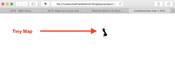
Open http://localhost:8008 in your favourite web browser.
Alternatively you can also use the Python http server:
python -m SimpleHTTPServer
Note: If Chrome shows this error in the JS console ` Uncaught TypeError: Cannot read property ‘type’ of undefined
then you are referencing an object that doesn't exist in your topology. ([Source](http://stackoverflow.com/questions/15509493/topojson-js187-uncaught-typeerror-cannot-read-property-type-of-undefined)). **Firefox** displayed the same error as:TypeError: t is undefined`.
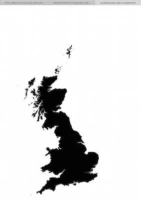
Once the page is loaded in your favourite web browser, you will see a very small map.
Let’s scale the map now and also change the projection type:
var width = 960,
    height = 1160;

var projection = d3.geo.albers()
//var projection = d3.geo.mercator()
    .center([0, 55.4])
    .rotate([4.4, 0])
    .parallels([50, 60])
    .scale(4000)
    .translate([width / 2, height / 2])
    //.translate(200,200)
    ;

var path = d3.geo.path()
    .projection(projection);

var svg = d3.select("body").append("svg")
    .attr("width", width)
    .attr("height", height);

d3.json("constituencies.topo.json", function(error, topology) {
    svg.append("path")
        // convert topojson back to geojson
        .datum(topojson.feature(topology, topology.objects.constituencies))
        .attr("d", path);
});
The result should look like this:
Color Coding
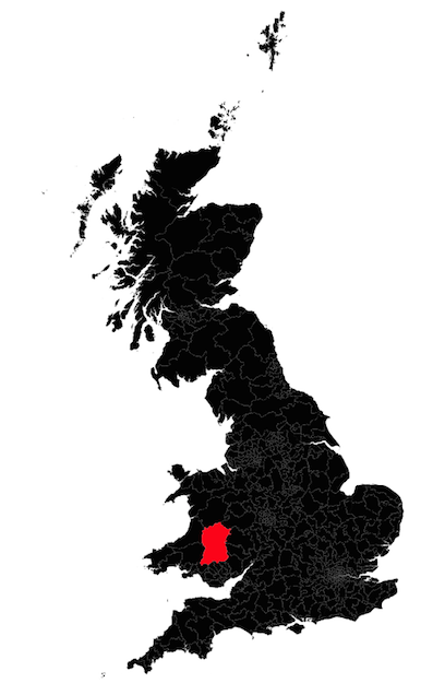
Highlighting one Constituency
We’d like to color code the constituencies in a specific color. Let’s start in a simple fashion and just try to assign a static color to a given constituency.
To make this happen, we have to change the way the map is drawn: We have to create a polygon for each constituency and store the value of id in a newly created constituency property:
d3.json("constituencies.topo.json", function(error, topology) {
  // create a polygon for every constituency
  svg.selectAll(".constituency")
    // retrieve the features so that we can access the id
    	.data(topojson.feature(topology, topology.objects.constituencies).features)
    	.enter().append("path")
    	.attr("class", function(d) { return "constituency " + d.id; })
    	.attr("d", path);
});
We will highlight a bigger constituency (Brecon and Radnorshire), so that the effect is easy to spot. Amend the style section as follows:
<style>
.constituency.W28 { fill: red; }
</style>
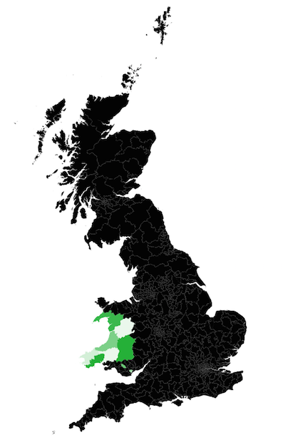
Highlighting multiple Constituencies
Now that we know how to highlight one constituency, we are eager to apply colours to more of them. We will still keep it relatively simple by just creating an array of constituency codes and associated colour codes. Although our array is static, it would be fairly easy to replace it by a dynamic data source.
Remove any CSS styles from our HTML document. Then adjust the JavaScript section as follows:
var data = [
    ['W28','rgba(23, 177, 48, 1)']
    ,['W12','rgba(23, 177, 48, 0.7)']
    ,['W11','rgba(23, 177, 48, 0.5)']
    ,['W10','rgba(23, 177, 48, 0.3)']
    ,['W9','rgba(23, 177, 48, 0.2)']
    ,['W8','rgba(23, 177, 48, 0.1)']
    ,['W27','rgba(23, 177, 48, 0.1)']
    ,['W24','rgba(23, 177, 48, 0.6)']
    ,['W23','rgba(23, 177, 48, 0.1)']
    ,['W21','rgba(23, 177, 48, 0.9)']
    ,['W26','rgba(23, 177, 48, 1)']
    ,['W25','rgba(23, 177, 48, 0.2)']
]
;

// create map
var width = 700,
    height = 1000;

var projection = d3.geo.albers()
    //.center([0, 55.4])
    .center([3, 54])
    .rotate([4.4, 0])
    .parallels([50, 60])
    .scale(4000)
    .translate([width / 2, height / 2])
    //.translate(200,200)
    ;

var path = d3.geo.path()
    .projection(projection);

var svg = d3.select('body').append('svg')
    .attr('width', width)
    .attr('height', height);

d3.json('constituencies.topo.json', function(error, topology) {
    // create a polygon for every constituency
    svg.selectAll('.constituency')
    // retrieve the features so that we can access the id
    	.data(topojson.feature(topology, topology.objects.constituencies).features)
    	.enter().append('path')
    	.attr('class', function(d) { return 'constituency ' + d.id; })
    	.attr('d', path)
    	;

    //svg.select('.W28').attr('fill','red');

    // dynamic coloring
    data.forEach(function(elt, i) {
      console.log(elt[0] + ': ' + elt[1]);
      console.log(svg.select(elt[0]));
      svg.select('.' + elt[0]).attr('fill',elt[1]);
    });
});
Dynamic Color Coding
A primitive approach
Now we will replace the color codes in our data array by the actual measures. As a first try we can write our own primitive function, which returns a suitable color code for a given measure:
var myData = [
	['W28',3223534]
	,['W12',234255]
	,['W11',2352332]
	,['W10',563452]
	,['W9',234]
	,['W8',563432]
	,['W27',23455]
	,['W24',462342]
	,['W23',978465]
	,['W21',67456]
	,['W26',1232543]
	,['W25',764343]
]
;

// dynamic color shades
var measures = [];

myData.forEach(function(elt, i) {
  measures.push(elt[1]);
})
;

var countItmes = myData.length;
var measuresMin = Math.min.apply(Math,measures);
var measuresMax = Math.max.apply(Math,measures) + 1; // added plus 1 so that we can use >= and < in range checks further down
var range = measuresMax - measuresMin;
var unit = range / countItmes;
var ranges = [];

for(i=0;i<countItmes;i++){
    var range = [];
    // min
    range.push(measuresMin + (unit * i));
    // max
    range.push(measuresMin + (unit * (i+1)));
    // color: opacity must not be lower than 0.1
    // not really the best algorithm, but it works for now
    range.push('rgba(23, 177, 48, ' + ( 0.1 + ((0.9 / countItmes) * ( i + 1 ) )) + ')');
    ranges.push(range);
}

myData.forEach(function(row, i) {
    ranges.forEach(function(elt, z) {
        if( row[1] >= elt[0] && row[1] < elt[1] ) {
            // add range color to dataset
            // console.log('The value ' + row[1] + 'falls between ' + elt[0] + ' and ' + elt[1]);
            row.push(elt[2]);
        }
    });
});

// create map
var width = 700,
    height = 1000;

var projection = d3.geo.albers()
    //.center([0, 55.4])
    .center([3, 54])
    .rotate([4.4, 0])
    .parallels([50, 60])
    .scale(4000)
    .translate([width / 2, height / 2])
    //.translate(200,200)
    ;

var path = d3.geo.path()
    .projection(projection);

var svg = d3.select('body').append('svg')
    .attr('width', width)
    .attr('height', height);

d3.json('constituencies.topo.json', function(error, topology) {
  // create a polygon for every constituency
  svg.selectAll('.constituency')
    // retrieve the features so that we can access the id
    .data(topojson.feature(topology, topology.objects.constituencies).features)
    .enter().append('path')
    .attr('class', function(d) { return 'constituency ' + d.id; })
    .attr('d', path)
    ;

    // add colors
    myData.forEach(function(elt, i) {
        svg.select('.' + elt[0]).attr('fill',elt[2]);
    });

});
Use existing and intelligent dynamic colour coding function
Why reinvent the wheel if there is already a colour coding function out there - one that is far better then the primitive function we just wrote above?
We can use the d3.scale.quantize() function in combination with ColorBrewer (See Ordinal-Scales article and in particular the ColorBrewer section at the end of this article. Mike Bostock provided an example, and the code is available here.).
<!DOCTYPE html>
<html>
    <head>
        <meta charset='utf-8'>
        <style>
/* color codes for our map */
.q0-9 { fill:rgb(247,251,255); }
.q1-9 { fill:rgb(222,235,247); }
.q2-9 { fill:rgb(198,219,239); }
.q3-9 { fill:rgb(158,202,225); }
.q4-9 { fill:rgb(107,174,214); }
.q5-9 { fill:rgb(66,146,198); }
.q6-9 { fill:rgb(33,113,181); }
.q7-9 { fill:rgb(8,81,156); }
.q8-9 { fill:rgb(8,48,107); }
        </style>
    <body>
        <script src="https://cdnjs.cloudflare.com/ajax/libs/d3/3.5.5/d3.min.js"></script>
        <script src="https://cdnjs.cloudflare.com/ajax/libs/topojson/1.6.19/topojson.min.js"></script>
        <script>

var myData = [
    ['W28',3223534]
    ,['W12',234255]
    ,['W11',2352332]
    ,['W10',563452]
    ,['W9',234]
    ,['W8',563432]
    ,['W27',23455]
    ,['W24',462342]
    ,['W23',978465]
    ,['W21',67456]
    ,['W26',1232543]
    ,['W25',764343]
]
;

// create map

var width = 700,
    height = 1000;

var myDataMin = d3.min(myData, function(d, i) { return myData[i][1]; });
var myDataMax = d3.max(myData, function(d, i) { return myData[i][1]; });
// d3.max(data, function(d) { return d.votes; })

console.log('The range of my data is: ' + myDataMin + ' - ' + myDataMax);

var quantize = d3.scale.quantize()
    .domain([myDataMin, myDataMax])
    .range(d3.range(9).map(function(i) { return "q" + i + "-9"; }))
    // Note 9 define in the range() function relates to the 9 CSS styles we defined above
    ;

var projection = d3.geo.albers()
    //.center([0, 55.4])
    .center([3, 54])
    .rotate([4.4, 0])
    .parallels([50, 60])
    .scale(4000)
    .translate([width / 2, height / 2])
    //.translate(200,200)
    ;

var path = d3.geo.path()
    .projection(projection);

var svg = d3.select('body').append('svg')
    .attr('width', width)
    .attr('height', height);

d3.json('constituencies.topo.json', function(error, topology) {
    // create a polygon for every constituency
    svg.selectAll('.constituency')
    // retrieve the features so that we can access the id
        .data(topojson.feature(topology, topology.objects.constituencies).features)
        .enter().append('path')
        .attr('class', function(d) { return 'constituency ' + d.id; })
        .attr('d', path)
        ;

    // add colors
    myData.forEach(function(elt, i) {
        //console.log(elt[0] + ': ' + elt[1] + ' -> color: ' + quantize(elt[1]));
        svg.select('.' + elt[0]).attr('class', quantize(elt[1]));
    });
});

        </script>
    </body>
</html>
Now that we have figured out how to create a map and dynamically colour code the constituencies, we are mostly ready to publish to map to a server. We will go at least on step further and dynamically feed in the data, so that we can see the UK General Election Results 2015. This will be covered in the next article, where we will take a look at integrating our D3 code with a dashboard on the Pentaho BA Server.